

1. INTRODUCTION
2. MATERIAL
2.1 Data description
2.2 Artificial neural networks (ANN)
2.3 Adaptive neuro-fuzzy inference system (ANFIS)
2.4 Wavelet-based neural networks (WNN)
2.5 Genetic algorithm (GA)
2.6 K-fold cross validation (CV)
3. METHODOLOGY
3.1 Models development
3.2 Coding for the ANN, ANFIS, and WNN models
3.3 Measures of accuracy
4. Results and Discussion
5. Conclusion
1. INTRODUCTION
Streamflow forecasting based on accurate measurements can be used to design flood mitigation structures for agricultural and urban basins, and build water allocation systems for agricultural, industrial, and commercial purposes (Rezaie-Balf et al., 2019; Samsudin et al., 2011). The complex and significant variability of streamflow can be explained using spatial and temporal characteristics. It has guided the evolution and application of different approaches for estimation, modeling, forecasting, and prediction (Martins et al., 2011). Forecasting of hydrological time series (e.g., streamflow, water stage, evaporation, and groundwater stage etc.) is important for understanding the internal relationship of natural processes (Krishna et al., 2011). Since the complexity of hydrological time series requires specific tools of non-linear and non-stationary dynamic systems, the diverse forecasting methods have been proposed for hydrological forecasting (Sivakumar et al., 2001).
Data-driven approaches, although credible for hydrological forecasting, don’t have the capability to depict physical processes, because they only consider an adequate selection of hydrological variables with temporal and input-output modification. Therefore, these approaches can be categorized as two types (i.e., classicial and computational intelligence approaches) typically. The classical approaches can be exemplified as linear regression (LR), auto regressive integrated moving average (ARIMA), and ARIMA with exogenous input (ARIMAX) etc. The machine learning approaches can be classified as artificial neural networks (ANN), adaptive neuro-fuzzy inference systems (ANFIS), genetic programming (GP), gene expression programming (GEP), model tree (MT), extreme learning machines (ELM), support vector machines (SVM), and multivariate adaptive regression spline (MARS) etc. The field of machine learning approaches has undergone innovative changes for novel techniques of data simulation and processing (Chandwani et al., 2015).
For three decades, the ANN model based on neuron systems has been used for different types of hydrological forecasting. Various approaches have been applied to validate the accuracy and effectiveness of the ANN model for streamflow forecasting (Biswas and Jayawardena, 2014; Badrzadeh et al., 2013; Moradkhani et al., 2004; Cigizoglu, 2003; Abrahart and See, 2000). The ANFIS model (Jang, 1993), which has the merits of the ANN model and the fuzzy system, has been employed for streamflow forecasting (Talei et al., 2010; Nasr and Bruen, 2008; Keskin et al., 2006; Lohani et al., 2006).
Methodologies combining wavelet and machine learning approaches have been utilized for streamflow forecasting. Combined approaches have outstripped conventional models (Nourani et al., 2014). The wavelet-based machine learning approaches, including wavelet-based neural networks (WNN), wavelet-based support vector regression (WSVR), and wavelet-based adaptive neuro fuzzy inference system (WANFIS), have been effectively implemented for hydrological forecasting, including streamflow, water stage, runoff, and groundwater etc. (Seo et al., 2015; Kamruzzaman et al., 2013; Partal, 2009; Partal and Kisi, 2007). Many researchers have attempted to forecast streamflow using wavelet-based machine learning approaches (Zakhrouf et al., 2016, 2020; Shoaib et al., 2014; Badrzadeh et al., 2013; Nourani et al., 2013; Guo et al., 2011; Tiwari and Chatterjee, 2010).
The optimal structure of wavelet-based machine learning approaches can be constructed as a search method. A method for designing machine learning approaches using evolutionary optimization algorithm is proposed to format the best models. Evolutionary machine learning approaches for modeling hydrologic systems have been suggested by Zakhrouf et al. (2018), Kalteh (2015), Sahay and Srivastava (2014), Asadi et al. (2013).
K-fold cross validation (CV) method is one of the methods to assess the algorithmic generalization. The out-of-sample cross validation (OOS-CV) method is a frequently used method for hydrological modeling. This paper attempts to develop a new approach combining wavelet transformation, machine learning approach, evolutionary optimization algorithm, and k-fold cross validation method for multi-step (days) (i.e., t+1, t+2, and t+3 days) streamflow forecasting in the Seybous River, North Algeria. The paper is divided into five chapters. The first part provides a brief introduction. The second part discusses data and application tools, including ANN, ANFIS, WNN, GA, and k-fold CV, respectively. The third part applies the methodology, and results and discussion are presented in the fourth part. Conclusions are stated in the concluding part.
2. MATERIAL
2.1 Data description
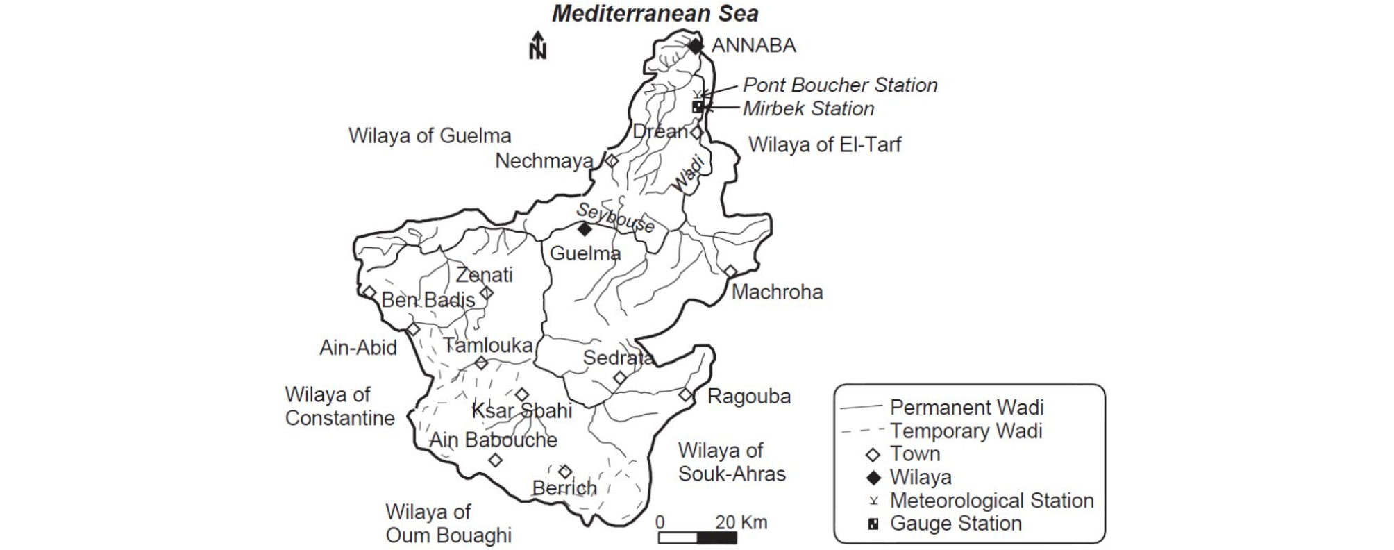
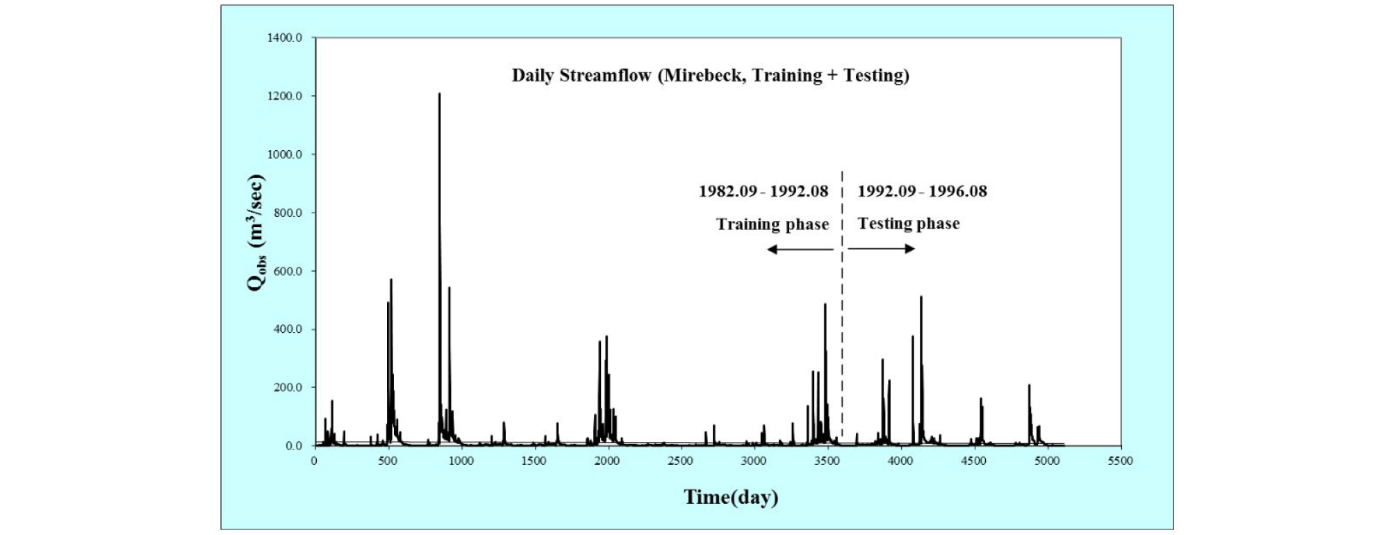
The data for training and testing phases of the developed models were obtained from the Seybous River basin, Algeria. The basin is positioned between 36.0 N and 38.0 N (latitudes), and between 7.0 E and 8.0 E (longitudes), Algeria, North Africa, and covers a total catchment area of 6,471.0 km2 (Fig. 1). Daily streamflow data for 14 years (September, 1982-August, 1996) were obtained from National Agency of Water Resources of Mirebeck (14 06 01) gauging station and were utilized for multi-step (days) streamflow forecasting. These selected multi-step (days) can be adequate, considering the rapid surface streamflow in the Mediterranean basin and the watershed size. For this purpose, the first ten years (70% of data) were utilized for the training phase, and the second four years (30% of data) were utilized for the testing phase as shown in Fig. 2.
2.2 Artificial neural networks (ANN)
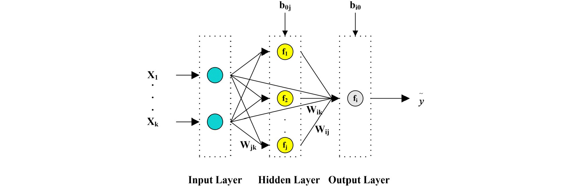
ANN is a parallel computational system based on the architectural and functional standard of biological networks (Imrie et al., 2000). The feedforward neural networks (FFNN) is one of the commonly applied neural network architectures. It consists of an input layer (i.e., first layer) which gets any outside news directly; an output layer (i.e., final layer); and one or more transitional layers (i.e., hidden layers) which divide the input and output layers. The neurons in the layers are usually fully connected using signs from the first layer to the final layer (Zhang et al., 1998), where the signs are handled by a consolidation function combining first all incoming signs, and second an activation function converting output neuron (Günther and Fritsch, 2010). Fig. 3 shows a conventional FFNN architecture.
2.3 Adaptive neuro-fuzzy inference system (ANFIS)
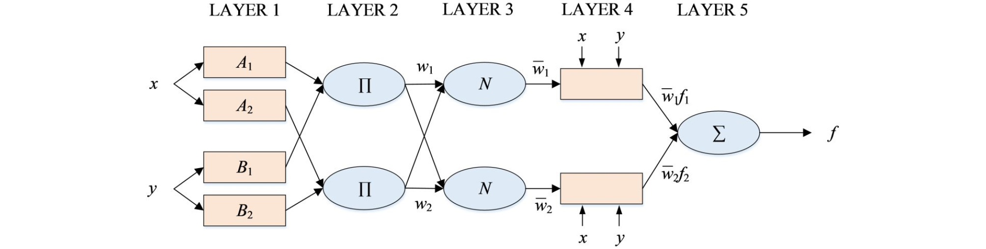
ANFIS is a complex function combining an adaptive neural network and a fuzzy inference system (FIS). The basic formation of a FIS consists of a structure that draws input to membership functions (Moosavi et al., 2013). Since ANFIS is based on FIS, it can be described using fuzzy IF-THEN rules (Jang et al., 1997). There are two methods for FIS: Mamdani (Mamdani and Assilian, 1975) and Sugeno (Takagi and Sugeno, 1985). The differences between the two methods can be explained using the consequent part. Mamdani’s method utilizes fuzzy membership functions (MFs), whereas Sugeno’s method applies linear or constant functions. In this study, the procedures presented by Jang et al. (1997) using Sugeno’s approach were utilized for multi-step (days) streamflow forecasting. Fig. 4 shows the conventional ANFIS architecture. The ANFIS was trained using the least-squares method (LSM) and backpropagation gradient descent method (BP-GDM). Detailed explanation for the ANFIS model can be found in Jang (1993).
2.4 Wavelet-based neural networks (WNN)
The fundamental objective of the wavelet transform (WT) is to finalize a complete time scale formation of localized and passing events happening at different time scales (Labat et al., 2000). There are two categories of WT: continuous wavelet transform (CWT) and discrete wavelet transform (DWT). The CWT method can be applied for continuous functions or time series (Nourani et al., 2009; Mallat, 1989). Since the CWT method is time-consuming, it requires large resources, whereas the DWT method can be more easily applied (Nourani et al., 2009; Mallat, 1989). The DWT requires less calculation time, is not complicated (Ghaemi et al., 2019; Quilty and Adamowski, 2018; Seo et al., 2015, 2018; Kisi, 2011; Nourani et al., 2009; Mallat, 1989), and involves choosing scales and positions (Adamowski and Sun, 2010).
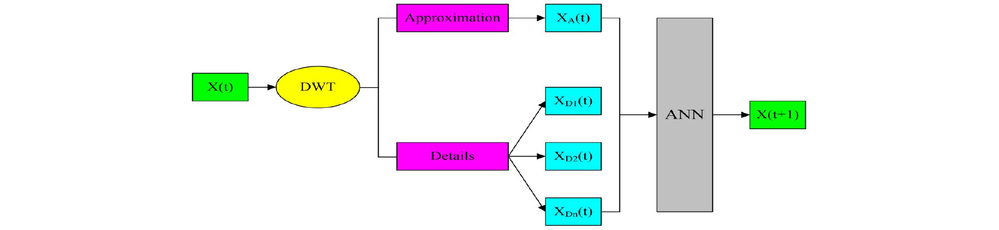
A WNN model is a combination of WT and ANN, where the original time series for each input neuron of the ANN model is decomposed to some multi-frequency time series using the WT algorithm. The decomposed details (D) and approximation (A) are formatted as new inputs to the ANN model architecture, as shown in Fig. 5. The WNN model consists of a two-stage algorithm. The first stage can be specialized with the multi-level WT where the original time series is decomposed utilizing the WT after choosing the decomposition level. The second stage can be classified as the training and testing phases using the ANN model. The details and approximation, which are obtained by the WT in the first stage, are utilized as input of the ANN model. In the WNN, the number of decomposition levels (details and approximation) of each input is calculated according to full data length (Nourani et al., 2009).
| $$L=int\lbrack log(N)\rbrack$$ | (1) |
where L defines the decomposition level, N denotes the number of time series data, and int[·] depicts the integer-part function. In this study, the data comprised N = 5110 samples; therefore, the level decomposition was classified as L = 3.
2.5 Genetic algorithm (GA)
GA, developed by Holland (1975), is a heuristic and evolutionary optimization technique based on evolutionary and genetic theory (Kim and Kim, 2008). The procedure of GA starts with random strings representing design or decision variables. Each string is then evaluated to allocate the fitness value, based on the objective and constraint conditions. Then, the termination condition is validated in the algorithm (Gowda and Mayya, 2014). This study focuses on optimizing the structure of three machine learning approaches (i.e., ANN, ANFIS, and WNN) using the evolutionary optimization algorithm (i.e., GA).
The first step is to choose the GA chromosome. Each individual in the population represents a possible configuration for architecture of the machine learning approach. Based on the concept of evolutionary optimization theory, GA starts with a population of chromosomes, which evolve towards optimum solutions by GA operators, including selection, crossover, and mutation. These steps are reiterated from one generation to the next with the aim of arriving at the general optimal solution (Kim and Kim, 2008).
2.6 K-fold cross validation (CV)
The CV is a statistical methodology for comparing and evaluating training algorithms by separating data into two parts. One is utilized to train a model and the other is utilized to test it (Stone, 1974). K-fold CV assesses the generalization of algorithms in the evolutionary machine learning approach. Based on the category of k-fold CV, the data is first separated into k equally measured parts. Subsequently, k iterations of training and testing phases are performed such that a different part of the data is held-out for testing phase within each iteration, while the remaining (k-1) parts are used for training phase (Zhao et al., 2018)
Suppose we have a model with one or more unknown parameters f (), and a data set to which the model can be fitted. The primary method to estimate the tuning parameter using k-fold CV divides the data into rougher parts (Fig. 6). Since the model computes the mean squared error (MSE) for each i= 1, 2, …, k, the cross validation error (CVE) can be calculated as Eq. (2).

| $$CVE(\alpha)=\frac1K\sum_{i=1}^kMSE_i(\alpha)$$ | (2) |
where CVE defines the cross validation error.
3. METHODOLOGY
3.1 Models development
The machine learning approaches (i.e., ANN, ANFIS, and WNN) were utilized for multi-step (days) streamflow forecasting using previous time series values. The training phase of machine learning approaches provides a non-linear matching between inputs and outputs, and is useful in identifying patterns utilizing complicated data (Liu and Chung, 2014). Since the backpropagation (BP) algorithm cannot be guaranteed to find the minimum error margin, the convergence cannot occur with fast track. The solution for this problem can be applied with a fitness function that tests how well an architecture learns from the data. The fitness function can be expressed as Eq. (3).
| $$F=Min\lbrack CVE\rbrack$$ | (3) |
where F denotes the fitness function. In general, GA can significantly reduce the weakness of BP algorithm. The data utilized for the training phase (the 75% of the data) were sub-divided into 10 subsets (10-fold cross validation). Real coding was utilized to find the favorable topology for the ANN, ANFIS, and WNN models. The coding to find the best architecture and parameters of machine learning approaches (i.e., ANN, ANFIS, and WNN) is described as follows.
3.2 Coding for the ANN, ANFIS, and WNN models
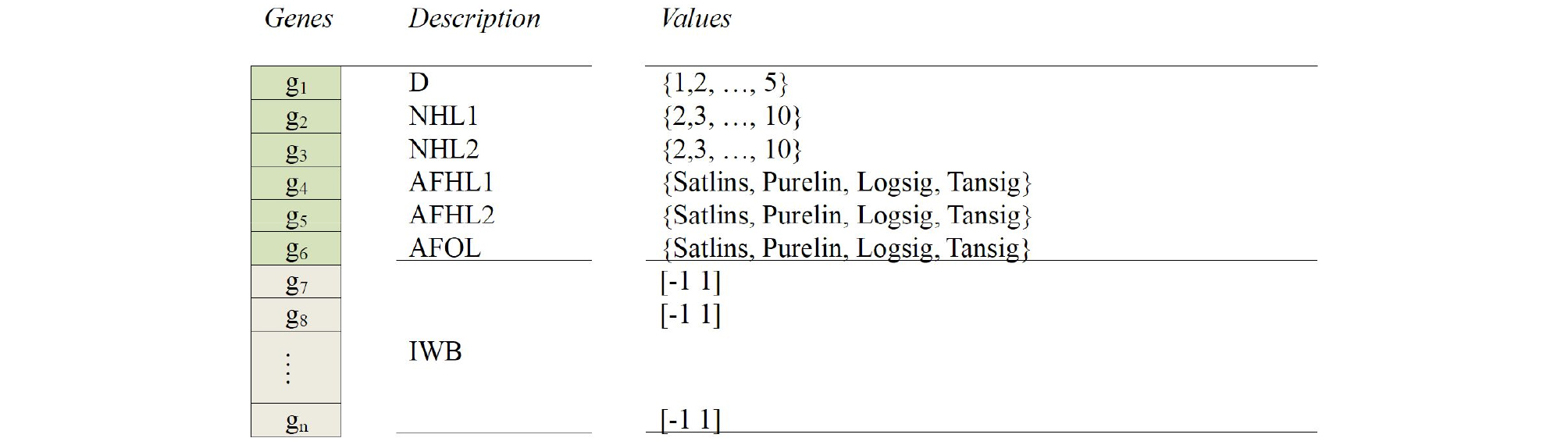
Feedforward neural networks (FFNN) models with two hidden layers and one neuron in final layer were utilized. A chromosome was built from a series of genes (Fig. 7) to find: the input delay (D), the number of neuron in the hidden layers (NHL1 and NHL2), the activation functions in the hidden and final layers (AFHL1, AFHL2, and AFOL) including linear transfer function (Purelin), symmetric saturating linear transfer function (Satlins), log-sigmoid transfer function (Logsig), and hyperbolic tangent sigmoid transfer function (Tansig), respectively, and the initial connection coefficients of weights and bias (IWB).
A chromosome of ANFIS model using a series of genes was created to find different parameters (Fig. 8): the input delay (D); the number of membership functions (NMF); the type of membership functions (TMF) including Π-shaped (Pimf), Trapezoidal-shaped (Trapmf), Triangular-shaped (Trimf), Gaussian curve (Gaussmf), and Built-in Gaussian function (Dsigmf); the definition of if-then (AND operation/OR operation) rules type (DRT); and the firing strength of a rule (FSR).

In this study, two methods were used as firing strength of AND rule, including Minimum (Min) and Product (Prod). Also, two methods were used as firing strength OR rule, including Maximum (Max) and the probabilisticOr method (Probor). For the membership functions type, there are many kinds of membership functions (MFs).
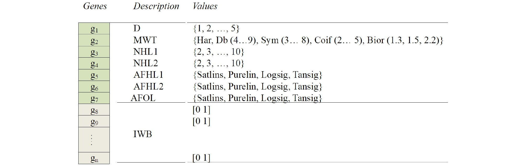
A chromosome of different parameters for wavelet-based neural networks (WNN) model was created from a series of genes (Fig. 9) to find: the input delay (D); the type of mother wavelet (TMW) based on the five most frequently used wavelet families, including Haar (Har), Daubechies (Db), Coiflets (Coif), Symlets (Sym), and Biorthogonal (Bior); the number of neuron in hidden layers (NHL1 and NHL2); the activation functions in hidden and output layers (AFHL1, AFHL2, and AFOL), including linear transfer function (Purelin), symmetric saturating linear transfer function (Satlins), log-sigmoid transfer function (Logsig) and hyperbolic tangent sigmoid transfer function (Tansig); and the initial connection weights and bias coefficients (IWB).
3.3 Measures of accuracy
To assess the performance of three different machine learning approaches (i.e., ANN, ANFIS, and WNN) to forecast multi-step (days) streamflow during the testing phase, four statistical indices (measures of accuracy) were applied, including root mean square error (RMSE), Nash-Sutcliffe efficiency (NSE), correlation coefficient (R), and peak flow criteria (PFC).
RMSE would vary from zero to a large value which presents prefect forecasting by the difference between observed and forecasted streamflow. NSE is considered for evaluating the ability of hydrological models (Rezaie-Balf et al., 2019; Nash and Sutcliffe, 1970). R is an assessment of the precision of hydrologic modeling and is used for comparisons of alternative models. A perfect matching produces R = 1.0 (Kim and Kim, 2008).
These statistical indices (i.e., RMSE, NSE, and R) may not provide the model performance for extreme streamflow events (e.g., floods and drought). Therefore, it is fundamental to evaluate the extreme distributions using PFC for forecasting extreme events (Rezaie-Balf et al., 2019). PFC plays an important role in following the extreme events to achieve the efficient model. The RMSE, NSE, R, and PFC indices can be represented as Eqs. (4)~(7).
| $$RMSE=\sqrt{\frac1N\sum_{i=1}^N\left[Qt_i-\widehat Qt_i\right]^2}$$ | (4) |
| $$NSE=\left(1-\frac{{\displaystyle\sum_{i=1}^n}\left[Qt_i-\widehat Qt_i\right]^2}{{\displaystyle\sum_{i=1}^N}\left[Qt_i-\overline Qt_i\right]^2}\right)\times100$$ | (5) |
| $$PFC=\frac{\sqrt[4]{{\displaystyle\sum_{i=1}^{T_p}}\left[Qt_i-\widehat Qt_i\right]^2\cdot Qt_i^2\;}}{\sqrt{{\displaystyle\sum_{i=1}^{T_p}}Qt_i^2}}$$ | (7) |
where = the observed streamflow value, = the forecasted streamflow value, = the mean observed streamflow, = the mean forecasted streamflow, N = the number of data, Tp = the number of peak streamflow greater than one third of the observed mean peak streamflow.
4. Results and Discussion
Table 1 presents the optimal structure of ANN model using GA which can be found from table 1 for (t+1) day forecasting as follows; input delay = 3, number of neurons (1st hidden layer) = 9, number of neurons (2nd hidden layer) = 8, activation function (1st hidden layer) = log-sigmoid transfer function, activation function (2nd hidden layer) = linear transfer function, and activation function (final layer) = linear transfer function. For (t+2) day forecasting, the following can be suggested; input delay = 3, number of neurons (1st hidden layer) = 9, number of neurons (2nd hidden layer) = 8, activation function (1st hidden layer) = log-sigmoid transfer function, activation function (2nd hidden layer) = log-sigmoid transfer function, and activation function (final layer) = linear transfer function. For (t+3) day forecasting, the following can be provided; input delay = 5, number of neurons (1st hidden layer) = 5, number of neurons (2nd hidden layer) = 8, activation function (1st hidden layer) = symmetric saturating linear transfer function, activation function (2nd hidden layer) = log-sigmoid transfer function, and activation function (final layer) = linear transfer function.
Table 1.
The optimal structure for ANN model using GA
| ANN parameters | t+1 | t+2 | t+3 |
| D | 3 | 3 | 5 |
| NHL1 | 9 | 9 | 5 |
| NHL2 | 8 | 8 | 8 |
| AFHL1 | Logsig | Logsig | Satlins |
| AFHL2 | Purelin | Logsig | Logsig |
| AFOL | Purelin | Purelin | Purelin |
Table 2 shows the optimal structure of ANFIS model using GA which can be expressed from table 2 for (t+1) day forecasting as follows; input delay = 1, number of membership functions = 3, type of membership functions = Gaussian curve, firing strength of a rule = product, and definition of if-then rules type = and. For (t+2) day forecasting, the following can be suggested; input delay = 2, number of membership functions = 3, type of membership functions = trapezoidal-shaped, firing strength of a rule = product, and definition of if-then rules type = and. For (t+3) day forecasting, the following can be provided; input delay = 2, number of membership functions = 2, type of membership functions = Gaussian curve, firing strength of a rule = probabilisticOr, and definition of if-then rules type = or.
Table 2.
The optimal structure for ANFIS model using GA
| ANFIS parameters | t+1 | t+2 | t+3 |
| D | 1 | 2 | 2 |
| NMF | 3 | 3 | 2 |
| TMF | Gaussmf | Trapmf | Gaussmf |
| FSR | Prod | Prod | Probor |
| DRT | And | And | Or |
Table 3 proposes the optimal structure of WNN model using GA which can be supposed from table 3 for (t+1) day forecasting as follows; input delay = 4, type of mother wavelet = Symlets 7, number of neurons (1st hidden layer) = 5, number of neurons (2nd hidden layer) = 10, activation function (1st hidden layer) = log-sigmoid transfer function, activation function (2nd hidden layer) = log-sigmoid transfer function, and activation function (final layer) = linear transfer function. For (t+2) day forecasting, the following can be suggested; input delay = 4, type of mother wavelet = Daubechies 9, number of neurons (1st hidden layer) = 8, number of neurons (2nd hidden layer) = 10, activation function (1st hidden layer) = symmetric saturating linear transfer function, activation function (2nd hidden layer) = log-sigmoid transfer function, and activation function (final layer) = linear transfer function. For (t+3) day forecasting, the following can be provided; input delay = 5, type of mother wavelet = Symlets 6, number of neurons (1st hidden layer) = 8, number of neurons (2nd hidden layer) = 7, activation function (1st hidden layer) =linear transfer function, activation function (2nd hidden layer) = symmetric saturating linear transfer function, and activation function (final layer) = linear transfer function.
Table 3.
The optimal structure for WNN model using GA
| WNN parameters | t+1 | t+2 | t+3 |
| D | 4 | 4 | 5 |
| MWT | sym7 | db9 | Sym6 |
| NHL1 | 5 | 8 | 8 |
| NHL2 | 10 | 10 | 7 |
| AFHL1 | Logsig | Satlins | Purelin |
| AFHL2 | Logsig | Logsig | Satlins |
| AFOL | Purelin | Purelin | Purelin |
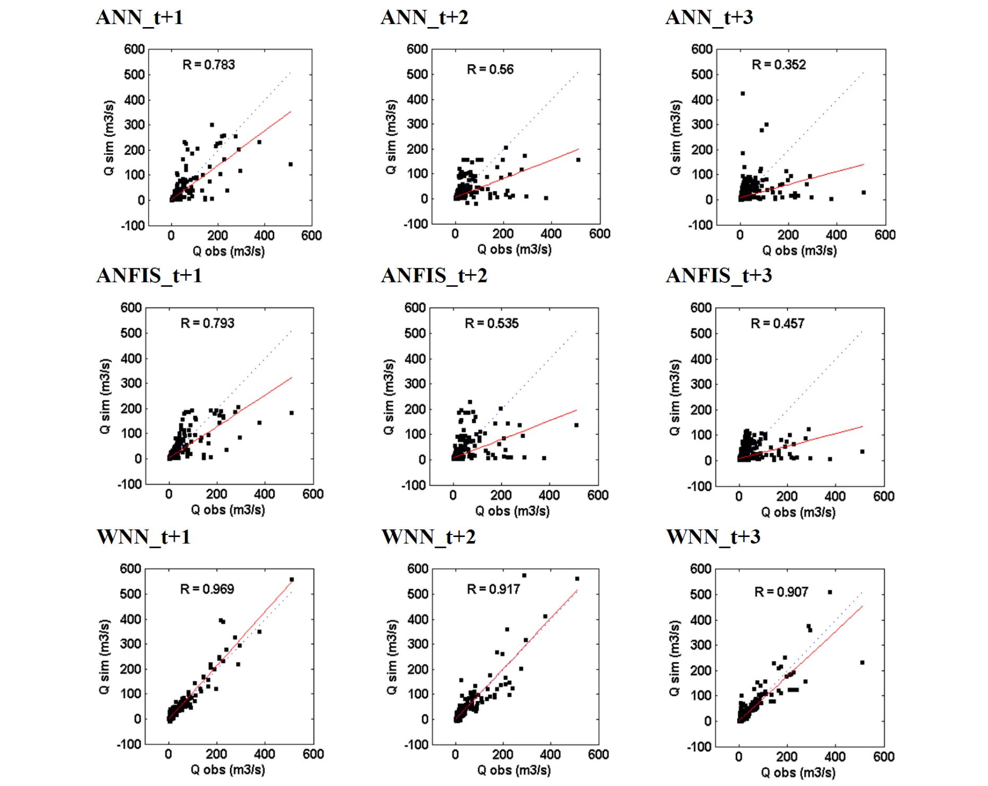
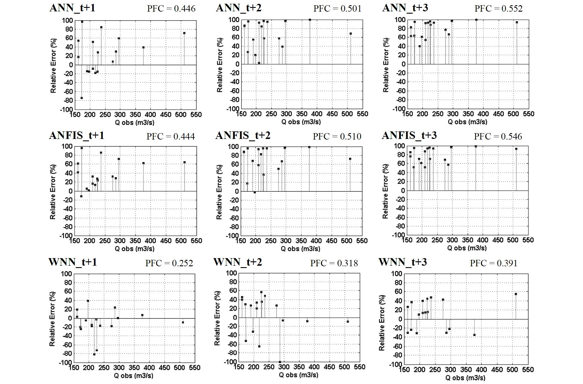
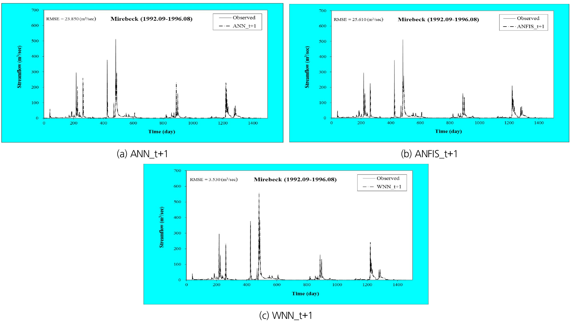
Table 4 suggests the performances of ANN, ANFIS, and WNN models for different multi-step (days) (i.e., t+1, t+2, and t+3 days) forecasting. The statistical results of standalone (i.e., ANN and ANFIS) models yielded similar performances based on RMSE, NSE, R, and PFC indices for training and testing phases. The performances of standalone models were not better than those of hybrid model (i.e., WNN). For example, the values of RMSE and PFC for the WNN model (RMSE = 8.590 m3/sec and PFC = 0.252, (t+1) day forecasting) were lower than those of ANN (RMSE = 19.120 m3/sec and PFC = 0.446, (t+1) day forecasting) and ANFIS (RMSE = 18.520 m3/sec and PFC = 0.444, (t+1) day forecasting) models in the testing phase. In addition, the values of NSE and R for the WNN model (NSE = 92.000% and R = 0.969, (t+1) day forecasting) were higher than those of ANN (NSE = 60.400% and R = 0.783, (t+1) day forecasting) and ANFIS (NSE = 62.860% and R = 0.793, (t+1) day forecasting) models in the testing phase. The performances of hybrid model were superior to those of standalone models.
As the multi-step (days) for the three models increased from (t+1) to (t+3) days, the model accuracy decreased. The hybrid model applied sub-time series by using WT as model input, while the standalone models utilized the original time series as model input without WT. It can be suggested from table 4 that the hybrid model using sub-time series as input data of the standalone models can improve the performance of conventional standalone models. Fig. 10 shows the scatter diagrams for the ANN, ANFIS, and WNN models in the testing phase. Fig. 11 presents the relative errors of peak flow for the ANN, ANFIS, and WNN models in the testing phase. Figs. 10 and 11 show that the performance of hybrid model was superior to that of standalone models. From the performance comparison, the performance of three models with (t+1) day was superior to that of (t+2) and (t+3) days. In addition, Figs. 12(a)~12(c) display the daily streamflow hydrographs for the ANN, ANFIS, and WNN models based on (t+1) day forecasting in the testing phase.
Table 4.
Comparison between the performance results obtained by the models: ANN, ANFIS, and WNN in the training and testing phases
The machine learning approaches were combined a data pre-processing technique and an evolutionary optimization algorithm based on k-fold cross validation. In addition, an attempt to do multi-step (days) streamflow forecasting is different compared to the previous studies (Rezaie-Balf et al., 2019; Seo et al., 2018; Zakhrouf et al., 2018; Abdollahi et al., 2017; Ravansalar et al., 2017; Zakhrouf et al., 2016). The forecasts confirmed the accuracy and effectiveness of developed models, based on the statistical indices and scatter diagrams. Different machine learning approaches (e.g., gene expression programming (GEP), support vector machines (SVM), extreme learning machines (ELM), model tree (MT), and multivariate adaptive regression spline (MARS) etc.) combined data pre-processing techniques (e.g., principal component analysis (PCA), maximum entropy spectral analysis (MESA), empirical mode decomposition (EMD), and ensemble empirical mode decomposition (EEMD) etc.) and evolutionary optimization algorithms (e.g., particle swarm optimization (PSO), ant colony optimization (ACO), harmony search (HS), tabu search (TS), and crow search algorithm (CSA) etc.) can also be pursued in further studies.
5. Conclusion
This study suggests three machine learning approaches, including artificial neural networks (ANN), adaptive neuro-fuzzy inference system (ANFIS), and wavelet-based neural networks (WNN) models for multi-step (days) streamflow forecasting in Seybous River basin, Algeria. The accuracy and effectiveness of developed models (i.e., ANN, ANFIS, and WNN) are evaluated based on four statistical indices, including root mean square error (RMSE), Nash-Sutcliffe efficiency (NSE), correlation coefficient (R), and peak flow criteria (PFC).
Based on the combination of evolutionary optimization algorithm and k-fold cross validation, the statistical results of hybrid (i.e., WNN) model are superior to those of standalone (i.e., ANN and ANFIS) models for different multi-step (days). Also, the results of (t+1) day streamflow forecasting are superior to those of (t+2) and (t+3) days, based on statistical indices and scatter diagrams. The combination of machine learning approach and data pre-processing technique based on the evolutionary optimization algorithm and k-fold cross validation can be a potential implement for accurate multi-step (days) streamflow forecasting. Hybrid methodologies combining diverse machine learning approaches and data pre-processing technique based on other evolutionary optimization algorithms and cross validations can be recommended for further studies.
