Exploring the power of physics-informed neural networks for accurate and efficient solutions to 1D shallow water equations

Van Gian Nguyen; Van Linh Nguyen; Sungho Jung; Hyunuk An; Giha Lee

doi:10.3741/JKWRA.2023.56.12.939

Preview

Research Article

Journal of Korea Water Resources Association. 31 December 2023. 939-953
https://doi.org/10.3741/JKWRA.2023.56.12.939

Exploring the power of physics-informed neural networks for accurate and efficient solutions to 1D shallow water equations

물리 정보 신경망을 이용한 1차원 천수방정식의 해석

Van Gian Nguyen^a

Van Linh Nguyen^b

Sungho Jung^c

Hyunuk An^d

Giha Lee^e^*

응웬 반지앙^a

응웬 반링^b

정 성호^c

안 현욱^d

이 기하^e^*

^aPh.D Student, Department of Advanced Science and Technology Convergence, Kyungpook National University, Sangju, Korea

^bPh.D Student, Department of Advanced Science and Technology Convergence, Kyungpook National University, Sangju, Korea

^cPostdoctoral Researcher, Disaster Prevention and Emergency Management Institute, Kyungpook National University, Sangju, Korea

^dAssociate Professor, Department of Agricultural. and Rural Engineering, Chungnam National University, Daejeon, Korea

^eProfessor, Department of Advanced Science and Technology Convergence, Kyungpook National University, Sangju, Korea

^a경북대학교 미래과학기술융합학과 박사과정

^b경북대학교 미래과학기술융합학과 박사과정

^c경북대학교 재난대응전략연구소 박사후연구원

^d충남대학교 지역환경토목학과 부교수

^e경북대학교 미래과학기술융합학과 교수

^{*Corresponding Author}

ABSTRACT

Shallow water equations (SWE) serve as fundamental equations governing the movement of the water. Traditional numerical approaches for solving these equations generally face various challenges, such as sensitivity to mesh generation, and numerical oscillation, or become more computationally unstable around shock and discontinuities regions. In this study, we present a novel approach that leverages the power of physics-informed neural networks (PINNs) to approximate the solution of the SWE. PINNs integrate physical law directly into the neural network architecture, enabling the accurate approximation of solutions to the SWE. We provide a comprehensive methodology for formulating the SWE within the PINNs framework, encompassing network architecture, training strategy, and data generation techniques. Through the results obtained from experiments, we found that PINNs could be an accurate output solution of SWE when its results were compared with the analytical method. In addition, PINNs also present better performance over the Artificial Neural Network. This study highlights the transformative potential of PINNs in revolutionizing water resources research, offering a new paradigm for accurate and efficient solutions to the SVE.

Keywords

Shallow water equations

Physics-informed neural networks

Artificial neural networks

천수방정식(shallow water equations, SWE)은 물의 거동을 수치적으로 해석하기 위한 지배방정식으로 수리수문 분야에 널리 활용되고 있으며, 비선형 연립방정식으로 일반적으로 수치적으로 해석할 수 있다. 하지만 기존의 여러 수치 해석법은 격자망 생성에 민감하며 복잡한 지형에서의 해석에 한계가 발생할 수 있다. 이러한 한계점을 극복하기 위하여 본 연구에서는 물리 정보 신경망(Physics-Informed Neural Networks, PINNs)을 사용하고자 하였다. PINNs은 물리 법칙을 신경망에 직접적으로 도입하여 지배방정식을 해석하고자 하는 기법이며 지배 방정식에 대한 물리적, 수학적 정보를 손실함수로 변환하여 최적화하고 해를 산정할 수 있다. 본 연구에서는 지배방정식을 PINNs 구조 내에서 사용할 수 있도록 신경망 구조, 학습 전략, 데이터 생성 기술과 같은 포괄적인 방법론을 제시하고 결과를 ANN 기법과 비교하였다. 물리적 사전지식이 반영되지 않은 ANN과 달리 PINNs은 천수방정식에 대하여 매우 정확한 수치적 솔루션을 효과적으로 제공하는 것으로 나타났다. 따라서 PINNs은 지배방정식의 수치해석적 연구에 많은 잠재력이 있는 것으로 판단되며, 정확하고 효율적인 천수방정식의 솔루션을 위한 기법으로 활용될 수 있을 것으로 기대된다.

키워드

천수방정식

물리 정보 신경망

인공신경망

MAIN

1. Introduction
2. Methodology
2.1 Shallow Water Equations (SWE)
2.2 Physics-informed Neural Networks (PINNs)
3. Experiments
3.1 Nonbreaking wave propagation
3.2 Dam breaking
3.3 Setting-up experiment
4. Results and Discussion
4.1 Dose the PINN method effectively approximate the outcomes of the conventional method?
4.2 How PINNs deal with the existence of discontinuous and shocking?
4.3 What are the comparative advantages of the PINN in contrast to the ANNs?
4.4 How does the spatial distribution of collection points influence the ultimate outcomes?
4.5 Limitations and Future Work
5. Conclusions

1. Introduction

The Shallow Water Equations (SWE)(de Saint-Venant, 1871) serve as a core mathematical model for describing the behavior of water flow in rivers, lakes, estuaries, and coastal regions (Bates et al., 2005; Hodges, 2019; Soares-Frazao et al., 2012). These equations, derived from the principles of conservation of mass and momentum, are widely used in hydrology, hydraulic and environmental engineering for predicting water levels, velocities, and the propagation of waves in such natural water systems (Bates et al., 2010; Ferrari et al., 2019; Van et al., 2016; Viero and Valipour, 2017).

Traditionally, numerical methods have been employed to solve SWE, such as finite difference (Kuffour et al., 2020; Lundgren and Mattsson, 2020), finite volume (An and Yu, 2014; Bermúdez et al., 1998; Cea and Bladé, 2015), and finite element methods (Ayog et al., 2021; Hai et al., 2008; West et al., 2017). Although these methods have made substantial contributions, they also demand greater effort and necessitate a profound comprehension of the inherent characteristics of SWE, including nonlinearity (Valiani and Caleffi, 2019), discontinuity, and shockwaves (Lu et al., 2020; Marras et al., 2018).

In recent years, machine learning (ML) and deep learning (DL) have received a lot of attention for the solution of partial differential equations (Beck et al., 2019; Han et al., 2018; Sirignano and Spiliopoulos, 2018). Furthermore, there have been also attempts to apply data-driven-based algorithms for the solutions of problems related to SWE (Guo et al., 2021; Kabir et al., 2020; Liu and Pender, 2015). In this type of approach, ML and DL are used to approximate the non-linear relationship between inputs and outputs obtained by numerical solver or simulated models. These models are generally referred to as surrogate models. However, one of the limitations of this approach is that the surrogate model often requires a sufficiently large amount of data in the training process (Vijayaraghavan et al., 2023). It could be computationally expensive to achieve data for training.

A novel computational framework has emerged, leveraging the power of physics-informed neural networks (PINNs), which combines the strengths of deep learning and governing physics equations to provide a robust and efficient approach to solving complex problems in various scientific and engineering problems (Lu et al., 2021; Mao et al., 2020; Raissi et al., 2019). One of the key advantages of PINNs is their ability to handle partial differential equations (PDE) with complex boundary conditions and spatiotemporal dynamics. Meanwhile, traditional numerical methods often struggle with high dimensionality, requiring significant computational resources and effort (Ni et al., 2020; Vacondio et al., 2014). In contrast, PINNs provide an elegant and efficient alternative by learning the underlying physics directly from data (Karniadakis et al., 2021). In addition, PINNs utilize automatic differentiation to represent differential operators, eliminating the explicit requirement for mesh generation (Cai et al., 2021). This data-driven approach circumvents the need for explicit analytical formulations or discretization schemes, making PINNs highly versatile and adaptable to a wide range of problems (Gao et al., 2021; Jagtap et al., 2022; Karniadakis et al., 2021; Lu et al., 2021; Zobeiry and Humfeld, 2021). Furthermore, through the inclusion of constraint PDEs in the loss function, the solutions obtained from PINNs are compelled to adhere to the underlying physics phenomena, facilitating their interpretability (Karniadakis et al., 2021; Ren et al., 2023; Xu et al., 2022).

Despite the substantial growth of research aimed at enhancing the PINNs algorithm, research on PINNs in the field of hydrology and water resources remains relatively scarce (Chen et al., 2023; Feng et al., 2023). Tartakovsky et al. (2020) proposed a PINNs method that estimates hydraulic conductivity in a subsurface flow environment. In a study by Bandai and Ghezzehei (2022), it was shown that PINNs employing locally layer-wise adaptive activation functions can yield solutions to the one-dimensional Richards’ equation that are comparable in accuracy to traditional numerical methods. The seamless integration of deep learning with SWE is also presented in previous studies. Feng et al. (2023) introduced a novel framework capable of assimilating diverse types of observations and directly solving the 1D Saint-Venant Equations. Notably, their study demonstrates the effectiveness of PINN-based downscaling, which incorporates observational data to generate more realistic subgrid solutions for along-channel water depth. The literature reviews discussed above highlight the potential efficacy of PINNs in approximating solutions to SWE. However, despite this potential promise, the widespread adoption of PINNs for solving the SWE system remains somewhat limited. Additionally, there is a distinct need for a deeper exploration of data-driven methodologies in approximating solutions to the SWEs. For instance, questions regarding the comparative efficiency of PINNs versus conventional Artifical Neural Network (ANN) models remain unaddressed. Moreover, the implications of data distribution on the accuracy and precision of PINNs model have yet to be systematically elucidated. This necessitates a comprehensive investigation into the performance and data sensitivity of PINNs in the context of SWE solutions.

As a consequence, the main objective of this paper is to explore the capabilities of PINNs for solving shallow water equations and to assess their effectiveness in accurately approximating water flow dynamics. We present a comprehensive methodology that encompasses the mathematical formulation of the SWE, the architecture and training strategy employed in PINNs, and the data generation techniques used for modeling training and validation. Our study endeavors to underscore the competence and efficacy of PINNs in accurately capturing and simulating fluid flow behavior. This investigation considers scenarios involving both steady flow conditions and instances characterized by highly pronounced fluctuations in flow. Initially, we analyze PINNs' capabilities concerning nonbreaking wave propagation experiments. Subsequently, we extend this assessment to a more intricate scenario involving the utilization of PINNs for simulating dam failure. Moreover, our study rigorously evaluates PINNs' ability to approximate solutions, employing comparisons with ANNs and examining the influence of data point distribution on the precision and reliability of the PINNs model outputs. Ultimately, this exploration accentuates the advantages and potentials inherent in the application of PINNs within fluid dynamics simulations.

The rest of the paper is formulated into the following sections: Section 2 presents briefly SWE and the structure of PINNs, Section 3 presents experiments in the current study, and Section 4 presents results and discussions. The main finding of the study will be concluded in Section 5.

2. Methodology

2.1 Shallow Water Equations (SWE)

The governing equations, represented by Eqs. (1) and (2), are derived from the 1D shallow water equations. These equations are a fundamental mathematical model and are generally utilized to describe the behaviors of water in the channels and rivers. The shallow water equations are derived from the principles of mass and momentum conservation, assuming incompressibility and negligible vertical velocities.

(1)

\frac{\partial h}{\partial t} + u \frac{\partial h}{\partial x} = 0

(2)

\frac{\partial u}{\partial t} + u \frac{\partial u}{\partial x} + g (\frac{\partial h}{\partial x} + S_{o}) + \frac{g n^{2} u^{2}}{h^{4 / 3}} = 0

In the given equations, $h$ represents the water depth (m), $u$ denotes the water velocity (m/s), $g$ corresponds to the acceleration due to gravity (m²/s), So represents the bed slope.

2.2 Physics-informed Neural Networks (PINNs)

In this study, the solutions of 1D-SWE are approximated by PINNs, instead of by numerical methods. Fig. 1 illustrates an artificial neural network (ANN) that takes spatiotemporal coordinates as input data and approximates the corresponding variables of interest in SWE.

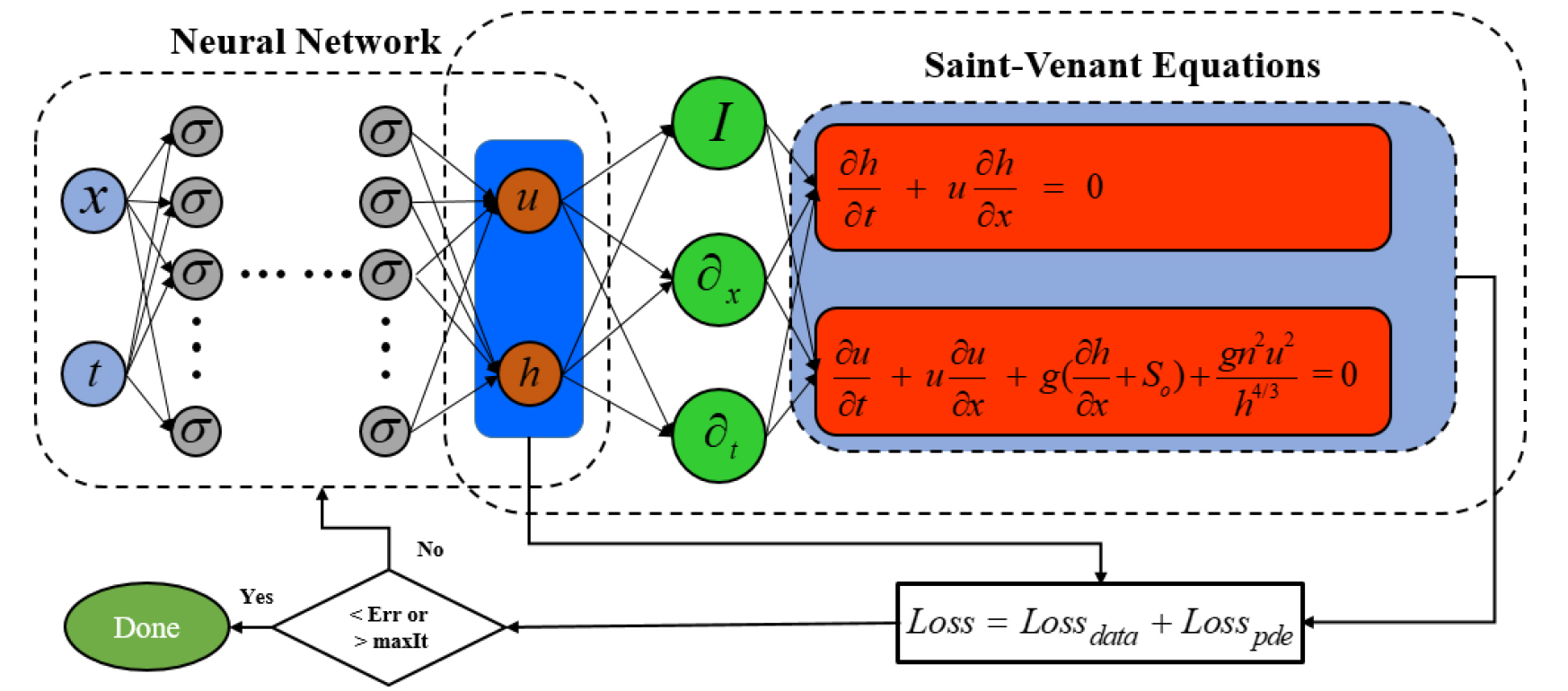
https://cdn.apub.kr/journalsite/sites/kwra/2023-056-12/N0200561210/images/kwra_56_12_10_F1.jpg

Fig. 1.

The diagram illustrates the configuration of PINNs for solving the SWE. On the left side, an uninformed neural network (NN), while on the right side, an informed NN is depicted, incorporating the conservation law. Both neural networks share the same set of hyperparameters and contribute to the overall loss function during training

Eq. (3) describes the fully connected nature of the neural network architecture employed in this study. The network consists of l hidden layers, with N neurons in each hidden layer. The inputs of the ith layer ( $Z_{l}$ ) are obtained by connecting the results of the previous layer ( $Z_{l - 1}$ ). This interconnected structure enables the flow of information throughout the network, facilitating the transformation and computation required to generate the desired outputs.

(3)

z_{l} = σ (W_{l} z_{l - 1} + b_{l})

The weight matrix ( $W_{l}$ ) and bias vector ( $b_{l}$ ) at the l^th layer are parameters that are determined through the training process. These parameters play a crucial role in the neural network's ability to capture the desired behavior. The activation function (𝜎) introduces nonlinearity to each output component, aiding in the network's ability to model complex relationships. In the current work, the tanh ( $x$ ) is selected as an activation function. The $W$ and $b$ are initialized using the Xavier scheme. The loss function presented in Eq. (4) includes two components. The first component involves the MSE between the ANN approximation and the boundary condition (BC) and initial condition (IC) data. The second component is the residuals of the PDEs, which are the summed residual errors of Eqs. (1) and (2) when using $u$ and $h$ as inputs. By incorporating both the PDE residuals and the data errors, this comprehensive loss function ensures that the network captures the governing physics and effectively approximates the solution to the problem, optimizing the network's performance.

(4)

L o s s = w_{1} L_{B C} (θ, N_{b}) + w_{2} L_{I C} (θ, N_{i}) + w_{3} L_{P D E} (θ, N_{f})

While $w_{1}, w_{2}$ , and $w_{3}$ present with weight loss of BC, IC, and PDE, respectively. The loss of each component in Eq. (4) is presented below:

(5)

{L_{B C}}_{u} (θ, {N_{b c}}_{u}) = \frac{1}{| {N_{b c}}_{u} |} \sum_{j = 1}^{{N_{b c}}_{u}} ∥ \hat{u} (x_{b c}^{j}, t_{b c}^{j}; θ) - u_{b c}^{j} ∥^{2}

(6)

{L_{B C}}_{h} (θ, {N_{b c}}_{h}) = \frac{1}{| {N_{b c}}_{h} |} ∥ \sum_{j = 1}^{{N_{b c}}_{h}} \hat{h} (x_{b c}^{j}, t_{b c}^{j}; θ) - h_{b c}^{j} ∥^{2}

(7)

{L_{I C}}_{h} (θ, {N_{i c}}_{h}) = \frac{1}{| {N_{i c}}_{h} |} ∥ \sum_{j = 1}^{{N_{i c}}_{h}} \hat{h} (x_{i c}^{j}, t_{i c}^{j}; θ) - h_{i c}^{j} ∥^{2}

(8)

L_{P D E} (θ, N_{f}) = \frac{1}{| N_{f} |} \sum_{j = 1}^{N_{f}} ∥ r_{f}^{2} (x_{f}^{j}, t_{f}^{j}; θ) ∥

The importance of weighting coefficients ( $w$ ) in the loss function (Eq. (4)) for training PINNs has been highlighted in previous studies (Feng et al., 2023; Wang et al., 2021). These coefficients play a crucial role in balancing the contributions of different loss terms, as an imbalance can hinder the convergence of the PINNs solution. Selecting appropriate weights is problem-dependent, as the optimal combination varies based on system properties and conditions. Typically, weights are tuned through trial-and-error procedures or empirically selected methods (Lee et al., 2022; Raissi et al., 2019; Zhang, 2022) because this method is relatively easy to implement. However, this method has been demonstrated to be time-consuming in looking for optimal parameters (Feng et al., 2023; Jin et al., 2021). Recently, McClenny and Braga-Neto (2020) have proposed a self-adaptive weight approach for automatically tuning the weights in the training process. Although, this method could provide acceptable accuracy, however, it also substantially increases the computational demand. To get out of the above situation, in this study, an effective method has been demonstrated in previous study (Chen et al., 2023; Feng et al., 2023; Wang et al., 2021) was adopted. This method employs dynamic weighting coefficients to scale various loss terms, ensuring balanced gradients during the back-propagation process of ANN training. The weighting coefficients are updated at each iteration of the training based on the previous iteration's loss (Loss). The formulation of the ANN parameters is defined by Eq. (9).

(9)

θ_{k + 1} = θ_{k} - η | \nabla_{θ} J_{f} (θ_{k}) + \sum_{j} \nabla_{θ} J_{j} (θ_{k}) |

The $w$ at the $(k + l)$ th iteration is calculated using the learning rate (𝜂) and the current iteration step ( $k$ ) according to the equation:

(10)

\hat{w_{j}} = \frac{\max x_{θ} | \nabla_{θ} J_{f} (θ_{k}) |}{\nabla_{θ} {\bar{J}}_{j} (θ_{n})}

The updated weighting coefficients are calculated using a moving average approach.

(11)

w_{j} = (1 - α) w_{j} + α {\hat{w}}_{j}

The hyperparameter $a$ , with a value of 0.9 as suggested by Feng et al. (2023) and Wang et al. (2021), controls the decay rate of the previous weight to maintain stability during training. The optimization of the DNN in PINNs is employed with the Adam optimizer. To facilitate convergence toward the correct solution, it is crucial to normalize the input data. Consequently, both spatial and temporal variables are mapped to the interval [-1, 1], where the input vector X corresponds to the concatenated value of $x$ and $t$ . This normalization step is essential to enhance the efficiency and accuracy of the PINNs model (Raissi et al., 2019).

(12)

X = \frac{2 X - \min (X)}{\max (X) - \min (X)} - 1

3. Experiments

As stated above, the main aim of this study is to explore the ability of PINNs to solve SWE. For that reason, the PINNs framework formulated in Section 2 will be applied to experiments. Specifically, a nonbreaking wave propagation problem (Bates et al., 2010; Feng et al., 2023; Hunter et al., 2005), which exists analytical solution under certain assumptions will be selected. After that, a comprehensive evaluation was carried out to compare the solution obtained from PINNs with the analytical solution.

3.1 Nonbreaking wave propagation

By considering flow over a planar surface, the continuity and momentum equations of the shallow water can be expressed in a simplified 1D form. Consequently, Eqs. (13) and (14) can be reformulated as follows:

(13)

\frac{\partial h}{\partial t} + u \frac{\partial h}{\partial x} = 0

(14)

\frac{\partial h}{\partial x} = - (S o + \frac{n^{2} u^{2}}{h^{4 / 3}})

Assuming a constant flow velocity over space and time, we can introduce a moving boundary condition where $h (u t, t)$ = 0 at $x = u t .$ Given that, $S_{0}$ = 0, the analytical solution for $h$ can be obtained by integrating the equation directly and incorporating the moving boundary condition.

This yields the following expression:

(15)

h (x, t) = - \frac{7}{3} [n^{2} u^{2} (x - u t)]^{3 / 7}

The boundary condition at $x$ = 0 is obtained from the analytical solutions:

(16)

h (0, t) = (\frac{7}{3} n^{2} u^{3} t)^{3 / 7}

For the simulation duration of 7200s, the reference solution in Eq. (15) is computed with the values u = 1 (m/s) and n = 0.01 (m^-1/3s).

3.2 Dam breaking

Dam-breaking involves the phenomena of the sudden release of stored water due to the failure or breach of a dam structure. In the event of a dam failure, the flow characteristics frequently manifest through phenomena such as discontinuities and shockwaves. For the 1D dam break simulation, the governing equations were described by Eq. (17).

(17)

\{\begin{cases} h_{t} + (h u)_{x} = 0 \\ (h u)_{t} + {(h u^{2} + \frac{1}{2} g h^{2})}_{x} = 0 \end{cases}

Where h is present for water depth (m), u is water velocity (m/s) and g is gravity acceleration. This study evaluates the ability of PINNs to simulate the behavior of the dam break problem. Specifically, how PINNs could be handled with the existence of discontinuities and shockwaves.

Fig. 2 depicts the schematic representation of a 1D dam structure employed for simulating dam failure. The simulation domain is confined within the x range of (-5, 5), and the temporal scope spans from t = 0 to t = 1. Initial conditions were prescribed as follows: h (x, 0) = 3 (m) for x less than or equal to zero, and h = 1 (m) for x greater than 0, with an initial velocity of 0(m/s). To assess the accuracy of PINNs in this scenario, we initially utilized a numerical method (Finite Volume Method) to approximate the solution in Eq. (17). Subsequently, PINNs were employed to track the flow dynamics associated with dam failure.

https://cdn.apub.kr/journalsite/sites/kwra/2023-056-12/N0200561210/images/kwra_56_12_10_F2.jpg

Fig. 2.

Schema for 1D dam failure simulation

3.3 Setting-up experiment

In our study, we investigated the performance of the PINNs model in approximating the 1D shallow water wave equation through a series of experiments. In Experiment 1, we constructed a PINNs framework with 6 hidden layers, each containing 64 neurons, to approximate the solution of the nonbreaking wave problem. This experiment provided valuable insights into the PINNs model's efficacy in this context. By using the identical manner as in Experiment 1, the accuracy of PINNs was investigated in situations existing shocking and discontinuous in Experiment 2. Furthermore, to understand the benefits of utilizing the PINNs model in comparison to the ANN model, we conducted Experiment 3. Notably, the structural configuration of the ANN model remained identical to that of the PINNs, with the sole exception being the inclusion of the governing equation. This comparative analysis shed light on the advantages of choosing the PINNs model over the conventional ANN approach. Additionally, the distribution of residual point collection within the domain of interest played a significant role in the performance of the PINNs model, as has been highlighted in prior research. In Experiment 4, we examined how the accuracy of the SWEs solution was influenced by the choice of collection point distribution. Two distinct collection point schemes, namely random sampling and selective sampling, were employed in this experiment to comprehensively understand the impact of data distribution on the accuracy of the PINNs model in approximating the SWEs.

The performance of the PINNs framework was assessed by calculating relative L2 error and root mean squared error (RMSE) using the following equations:

(18)

L 2 = \sqrt{\frac{\sum_{i = 1}^{N} (\hat{h_{i}} - h_{i})^{2}}{\sum_{i = 1}^{N} h_{i}^{2}}}

(19)

R M S E = \sqrt{\frac{1}{N} \sum_{i = 1}^{N} (\hat{h_{i}} - h_{i})^{2}}

where $\hat{h}$ and $h$ are the water level (m) estimated from PINNs (or ANN in Experiment 2) and analytical method, respectively.

4. Results and Discussion

In this section, the results of three experiments are presented and discussed, following the configurations described in Section 3.

4.1 Dose the PINN method effectively approximate the outcomes of the conventional method?

This first experiment serves to demonstrate the effectiveness of PINNs in solving simplified SWE with moving boundaries. The focus is on comparing the spatial-temporal evolution of water depth obtained from the analytical solution with PINNs.

By incorporating a limited set of IC and BC, along with the information from collection points within the calculation of the domain, PINN showcases its ability to accurately approximate the dynamic behavior of the water level. In addition, the results represented in Fig. 3 also indicate that PINNs can capture the underlying physics of the system and learn to simulate the evolution of water depth over time.

https://cdn.apub.kr/journalsite/sites/kwra/2023-056-12/N0200561210/images/kwra_56_12_10_F3.jpg

Fig. 3.

The dynamic of water level of (a) analytical method, (b) PINNs, and (c) is the difference between the analytical method and PINNs. The green, red, and black points are data of the initial, boundary, and collection conditions, respectively

By leveraging the flexibility and adaptability of PINNs, the comparison of water surface elevation presented in Fig. 4 indicates that PINNs are capable of effectively approximating the complex interactions and dynamics involved in the SWE problem with a moving boundary with almost insignificant differences. This allows for a more accurate representation of the real-world scenario compared to the traditional methods. In the field of hydrodynamics and coastal engineering, accurate predictions of water depth evolution are essential for designing and maintaining coastal structures, managing coastal erosion, and assessing flood risk. Furthermore, the relatively low difference which was plotted in Fig. 3(c) offers a new approach for various practical applications, and can potentially complement traditional methods, providing more efficient and accurate solutions for realistic applications.

https://cdn.apub.kr/journalsite/sites/kwra/2023-056-12/N0200561210/images/kwra_56_12_10_F4.jpg

Fig. 4.

Water surface elevation estimated from PINNs at different time steps

4.2 How PINNs deal with the existence of discontinuous and shocking?

Experiment 2 aims to assess the efficacy of PINNs in handling a particularly challenging scenario- the simulation of dam failure, known for its complexity and difficulty even for traditional numerical methods.

The disparity between the outcomes derived from the numerical method and the PINNs method appears negligible. Fig. 5 illustrates the spatiotemporal evolution of water depth. A comparative analysis between the PINN-derived outcomes and those from the numerical method reveals that the PINNs approach adeptly captures the overarching trends. Simultaneously, the diagrams displaying the spatial variation of water depth at different time intervals, as depicted in Figs. 5(c) and 5(d), underscore the capacity of PINNs to approximate solutions to the 1D SVEs equation. This is particularly notable in scenarios involving discontinuities and shock-like phenomena. Nonetheless, the visual examination in Fig. 5(b) underscores that the solution derived from the PINNs method does not encompass the entirety of water depth variations as comprehensively as the numerical method's outcomes. This distinction becomes particularly evident towards the conclusion of the simulation period and in the downstream region of the dam. The preceding analysis indicates that PINNs exhibit a commendable capacity in solving the SVE equation system. Nevertheless, in specific scenarios, such as those encountered in Experiment 2 of this study, where abrupt flow fluctuations arise, the accuracy of PINNs has not attained parity with solutions derived from numerical methods.

https://cdn.apub.kr/journalsite/sites/kwra/2023-056-12/N0200561210/images/kwra_56_12_10_F5.jpg

Fig. 5.

Spatial and temporal distribution of water depth from numerical method (NMM) (a); the water approximated by PINNs (b); The graph of water depth at t = 40 (s) and t = 100 (s) in (c) and (d), respectively. The green points and black points in (a) present for initial condition and residual points

4.3 What are the comparative advantages of the PINN in contrast to the ANNs?

The primary objective of this experiment is to evaluate and compare the performance of PINNs against ANN in terms of their respective merits. Specifically, the goal is to determine the merits of PINNs over ANN, which are renowned for their high performance and perceived difficulty to surpass in terms of accuracy. Fig. 6 displays the spatial and temporal distribution of input data for two models: ANNs (Fig. 6(a)) and PINNs (Fig. 6(b)). Green dots signify the initial condition, while red dots denote the boundary condition. Notably, the primary distinction between these models resides in their input data. While both models utilize initial and boundary conditions as inputs, the PINNs model integrates additional data from collection points to enhance the optimization of the loss function detailed in Eq. (5). Notably, the inter-model hyperparameters, such as model structure, activation function, and optimization function, are identical, facilitating a more straightforward assessment of their accuracy.

https://cdn.apub.kr/journalsite/sites/kwra/2023-056-12/N0200561210/images/kwra_56_12_10_F6.jpg

Fig. 6.

Presentation of training data with (a) for ANN, while (b) shows the collection points for training PINNs. The green, red, and black points are data of the initial condition, boundary condition, and collection points, respectively

Table 1 presents a comprehensive comparison of the performance between PINNs and ANNs for Experiment 2. The table includes essential details concerning the number of input data points utilized by both models. The results demonstrated in Table 1 clearly indicate that the PINNs model outperforms the ANN model. Notably, the most compelling evidence of superior performance lies in the significantly lower error achieved by the PINNs model, despite it having the same structure as the ANN model, except for constraint of PDE part. Specifically, the L2 error for ANN is 5.360e-2 (m), while the PINNs model achieves a lower L2 error of 3.638e-2(m). Furthermore, the RMSE for ANN is 0.041(m), whereas the PINNs model demonstrates a more favorable RMSE of 0.028(m). Based on the aforementioned analysis, the examination not only confirms the superior performance of the PINNs model over the ANN model but also sheds light on the underlying strengths of the PINNs approach. This prompts the question of the source of these advantages, given that both models share identical hyperparameters. The key lies in the additional information incorporated by the PINNs model, derived from collection points within the computational domain. This enriched dataset allows the PINNs model to optimize the solution of the SWE by effectively minimizing the loss function while considering the physical constraints imposed by the governing equations. By integrating the governing equations or physical principles as additional constraints, PINNs can effectively guide the learning process toward solutions that adhere to underlying physics (Karniadakis et al., 2021; Peng et al., 2021; Raissi et al., 2019). Various studies have consistently highlighted the limitations of ANN models in handling sparse data, leading to non-physical outcomes event when applied (Riley, 2019; Wang et al., 2020; Zobeiry and Humfeld, 2021). Furthermore, the reliance on a significant amount of labeled data during the training process further compounds the challenge, particularly in scientific machine-learning applications where such data ofter scarce (Gao et al., 2021; Sun and Wang, 2020). The finding of this experiment confirms the inherent advantage of PINNs in effectively approximating solutions to PDEs, exemplified by their successful application to SWE where PINNs’ solutions adhere to the laws of physics. Additionally, the results underscore the superiority of PINNs when faced with scenarios involving sparse training data, further highlighting the robustness and capability in handling data limitations.

Table 1.

Comparison between ANN and PINNs in terms of L2-norm and RMSE

Models	$N_{I C}$	$N_{B C}$	$N_{C}$	L2-norm (m)	RMSE (m)
ANN	5	10	-	5.360e-2	0.041
PINNs	5	10	500	3.638e-2	0.028

4.4 How does the spatial distribution of collection points influence the ultimate outcomes?

The final experiment in our study aims to address the question of how the results obtained from the PINNs model are influenced by different sampling methods for collection points within the computational domain. Two sampling methods are investigated in this experiment. The first method involves randomly drawing collection points, similar to Experiment 1, 2 and 3. In contrast, the second sampling method is specifically designed to target areas of high error in the calculation of domain. Based on observation from the results, it is evident that the errors of PINNs predominantly concentrate in the diagonal region of the computation domain. Consequently, collection points are deliberately selected around this high error region instead of employing random sampling. It is important to emphasize that the total number of input data points for the two PINNs in this experiment remains identical. The sole distinction lies in the distribution of the collection points.

Fig. 7(a) displays the spatial and temporal distribution of data points obtained through random sampling, whereas Fig. 7(b) showcases the deliberate selection sampling approach. Both models utilize an equal total number of collection points, with Nc = 720. Furthermore, the boundary condition and initial condition data points are specified as NBC = 10 and NIC = 5, respectively. Upon examining the outcomes of two PINNs models employing different sampling strategies, depicted in Figs. 7(c) and 7(d), the impact of the sampling strategy on the model results appears inconclusive. However, a notable distinction emerges when comparing the results obtained from PINNs with the analytical solution, as illustrated in Figs. 7(e) and 7(f). Evidently, when collection points are intentionally selected from the high-error region as input for PINNs, superior outcomes are achieved compared to randomly selected collection points.

https://cdn.apub.kr/journalsite/sites/kwra/2023-056-12/N0200561210/images/kwra_56_12_10_F7.jpg

Fig. 7.

Spatial distribution of collection points utilizing (a) random and (b) selective sample technique, the analytical solution of water depth (c and d), and the difference between analytical and PINNs methods corresponding to random and selective sample techniques (d and f)

The error indicators presented in Table 2 emphasize a more pronounced distinction between the two sampling strategies. In the case of the random selection strategy, the L2 error is reported as 2.748e-2(m) and the RMSE as 0.021(m). However, with the alternative sample selection strategy, the error indicators exhibit a significant reduction, with an L2 error of 1.645e-2(m) and an RMSE of 0.013(m). Upon comparing the outcomes presented in Experiment 1 and Experiment 4 concurrently, a discernible pattern emerges, underscoring the pivotal role of residual collection methods in augmenting the accuracy of the PINNs model. As shown by Fig. 8 regarding water level elevation at different times, it becomes evident that the utilization of a selective sampling approach yields results nearly indistinguishable from the analytical solution when employed in conjunction with the PINNs model.

Table 2.

Comparison between the random sample and selected sample schemes

Schemes	$N_{I C}$	$N_{B C}$	$N_{C}$	L2-norm (m)	RMSE (m)
Random	5	10	720	2.748e-2	0.021
Selected	5	10	720	1.645e-2	0.013

https://cdn.apub.kr/journalsite/sites/kwra/2023-056-12/N0200561210/images/kwra_56_12_10_F8.jpg

Fig. 8.

Water surface elevation at four selected time steps with selected sample schemes

The primary focus of PINNs lies in optimizing the PDE loss, ultimately guaranteeing the coherence between the trained network and the PDE under consideration (Karniadakis et al., 2021; Raissi et al., 2019). The PDE loss is assessed at a diverse array of scattered residual points. Consequently, the precise location and distribution of these residual points assume paramount importance in optimizing the performance of PINNs (Mao et al., 2020; Wu et al., 2023). Previous studies primarily employed a random uniform or nonuniform selection process for collection points, overlooking the importance of deliberate sample selection (Lu et al., 2021; Raissi et al., 2019; Tartakovsky et al., 2020). However, the results obtained in this study clearly indicate that the process of sample selection merits more careful consideration than simply randomly drawing residual points within the computational domain.

4.5 Limitations and Future Work

While the employed method in this study has demonstrated its effectiveness, it is important to acknowledge its limitations. The conducted experiments focused on relatively simple scenarios, calling for future research to expand the methodology to encompass more intricate and realistic situations, including complex topography and multiphase flow problems. Additionally, as the primary objective of this study was to assess the capability of PINNs in obtaining numerical solutions for SWE, the hyperparameters remained constant throughout the study. Thus, there is scope for refining the structure of PINNs, necessitating further investigations into hyperparameter optimization strategies to identify the most optimal configuration.

5. Conclusions

In this research, we have thoroughly investigated the application of Physics-Informed Neural Networks (PINNs) in estimating the solution of the 1D shallow water equations, with a specific focus on modeling the physics phenomena of non-breaking wave propagation over a flatbed. Our proposed approach leverages both measured data and the governing physical laws, creating a powerful synergy between empirical observations and mathematical constraints. Through three meticulously designed experiments, we have assessed the capabilities of PINNs and have drawn several key conclusions, which hold particular significance in the context of non-breaking wave phenomena:

1. PINNs have proven to be highly effective in providing numerical solutions for the 1D shallow water equations, accurately simulating the intricate dynamics of non-breaking wave propagation over a flatbed.

2. Unlike traditional Artificial Neural Networks (ANN), PINNs seamlessly integrate the governing physics knowledge into the training process, employing physics constraints within the loss functions. This unique characteristic allows us to represent the physical processes of wave behavior more faithfully.

3. PINNs have demonstrated clear advantages over traditional deep learning methods, particularly in situations with sparse data. This holds immense promise for applications where data may be limited, such as studying non-breaking wave phenomena in real-world scenarios. Nevertheless, further comprehensive investigation is required to ascertain the applicability of PINNs in scenarios characterized by abrupt and sudden alterations in flow dynamics.

4. Our experiments have unveiled that the distribution of collection points within the computational domain significantly influences the accuracy of the final solution, a critical insight for accurately modeling the non-breaking wave behavior over flatbeds.

Overall, this work represents a significant step toward harnessing the power of PINNs to model and understand complex physical phenomena, particularly in the context of non-breaking wave dynamics, and it sets a potential tool for future applications of the PINNs in real-world scenarios.

Acknowledgements

This work was supported by Korea Environmental Industry & Technology Institute (KEITI) through R&D Program for Innovative Flood Protection Technologies against Climate Crisis Project, funded by Korea Ministry of Environment (MOE)(2022003460002)

Conflicts of Interest

The authors declare no conflict of interest.

References

An, H., and Yu, S. (2014). "Finite volume integrated surface-subsurface flow modeling on nonorthogonal grids." Water Resources Research, Vol. 50, No. 3, pp. 2312-2328. 10.1002/2013WR013828

Ayog, J.L., Kesserwani, G., Shaw, J., Sharifian, M.K., and Bau, D. (2021). "Second-order discontinuous Galerkin flood model: Comparison with industry-standard finite volume models." Journal of Hydrology, Vol. 594, 125924. 10.1016/j.jhydrol.2020.125924

Bandai, T., and Ghezzehei, T.A. (2022). "Forward and inverse modeling of water flow in unsaturated soils with discontinuous hydraulic conductivities using physics-informed neural networks with domain decomposition." Hydrology and Earth System Sciences, Vol. 26, No. 16, pp. 4469-4495. 10.5194/hess-26-4469-2022

Bates, P.D., Dawson, R.J., Hall, J.W., Horritt, M.S., Nicholls, R.J., Wicks, J., and Hassan, M.A.A.M. (2005). "Simplified two-dimensional numerical modelling of coastal flooding and example applications." Coastal Engineering, Vol. 52, No. 9, pp. 793-810. 10.1016/j.coastaleng.2005.06.001

Bates, P.D., Horritt, M.S., and Fewtrell, T.J. (2010). "A simple inertial formulation of the shallow water equations for efficient two-dimensional flood inundation modelling." Journal of Hydrology, Vol. 387, No. 1-2, pp. 33-45. 10.1016/j.jhydrol.2010.03.027

Beck, C., E., W., and Jentzen, A. (2019). "Machine learning approximation algorithms for high-dimensional fully nonlinear partial differential equations and second-order backward stochastic differential equations." Journal of Nonlinear Science, Vol. 29, pp. 1563-1619. 10.1007/s00332-018-9525-3

Bermúdez, A., Dervieux, A., Desideri, J.-A., and Vázquez, M.E. (1998). "Upwind schemes for the two-dimensional shallow water equations with variable depth using unstructured meshes." Computer Methods in Applied Mechanics and Engineering, Vol. 155, No. 1-2, pp. 49-72. 10.1016/S0045-7825(97)85625-3

Cai, S., Mao, Z., Wang, Z., Yin, M., and Karniadakis, G.E. (2021). "Physics-informed neural networks (PINNs) for fluid mechanics: A review." Acta Mechanica Sinica, Vol. 37 No. 12, pp. 1727-1738. 10.1007/s10409-021-01148-1

Cea, L., and Bladé, E. (2015). "A simple and efficient unstructured finite volume scheme for solving the shallow water equations in overland flow applications." Water Resources Research, Vol. 51 No. 7, pp. 5464-5486. 10.1002/2014WR016547

Chen, Y., Xu, Y., Wang, L., and Li, T. (2023). "Modeling water flow in unsaturated soils through physics-informed neural network with principled loss function." Computers and Geotechnics, Vol. 161, 105546. 10.1016/j.compgeo.2023.105546

de Saint-Venant, A.J.-C. (1871). "Théorie du mouvement non-permanent des eaux, avec application aux crues des rivières et à l'introduction des marées dans leur lit." Academic de Sci. Comptes Redus, Vol. 73 No. 147-154, pp. 237-240.

Feng, D., Tan, Z., and He, Q. (2023). "Physics-informed neural networks of the Saint-Venant equations for downscaling a large-scale river model." Water Resources Research, Vol. 59 No. 2, e2022WR033168. 10.1029/2022WR033168

Ferrari, A., Viero, D.P., Vacondio, R., Defina, A., and Mignosa, P. (2019). "Flood inundation modeling in urbanized areas: A mesh-independent porosity approach with anisotropic friction." Advances in Water Resources, Vol. 125, pp. 98-113. 10.1016/j.advwatres.2019.01.010

Gao, H., Sun, L., and Wang, J.-X. (2021). "PhyGeoNet: Physics-informed geometry-adaptive convolutional neural networks for solving parameterized steady-state PDEs on irregular domain." Journal of Computational physics, Vol. 428, 110079. 10.1016/j.jcp.2020.110079

Guo, Z., Leitao, J.P., Simões, N.E., and Moosavi, V. (2021). "Data-driven flood emulation: Speeding up urban flood predictions by deep convolutional neural networks." Journal of Flood Risk Management, Vol. 14, No. 1, e12684. 10.1111/jfr3.12684

Hai, P.T., Masumoto, T., and Shimizu, K. (2008). "Development of a two-dimensional finite element model for inundation processes in the Tonle Sap and its environs." Hydrological Processes: An International Journal, Vol. 22, No. 9, pp. 1329-1336. 10.1002/hyp.6942

Han, J., Jentzen, A., and E.W. (2018). "Solving high-dimensional partial differential equations using deep learning." Proceedings of the National Academy of Sciences, Vol. 115, No. 34, pp. 8505-8510. 10.1073/pnas.171894211530082389PMC6112690

Hodges, B.R. (2019). "Conservative finite-volume forms of the Saint-Venant equations for hydrology and urban drainage." Hydrology and Earth System Sciences, Vol. 23, No. 3, pp. 1281-1304. 10.5194/hess-23-1281-2019

Hunter, N.M., Horritt, M.S., Bates, P.D., Wilson, M.D., and Werner, M.G. (2005). "An adaptive time step solution for raster-based storage cell modelling of floodplain inundation." Advances in Water Resources, Vol. 28, No. 9, pp. 975-991. 10.1016/j.advwatres.2005.03.007

Jagtap, A.D., Mao, Z., Adams, N., and Karniadakis, G.E. (2022). "Physics-informed neural networks for inverse problems in supersonic flows." Journal of Computational physics, Vol. 466, 111402. 10.1016/j.jcp.2022.111402

Jin, X., Cai, S., Li, H., and Karniadakis, G.E. (2021). "NSFnets (Navier-Stokes flow nets): Physics-informed neural networks for the incompressible Navier-Stokes equations." Journal of Computational physics, Vol. 426, 109951. 10.1016/j.jcp.2020.109951

Kabir, S., Patidar, S., Xia, X., Liang, Q., Neal, J., and Pender, G. (2020). "A deep convolutional neural network model for rapid prediction of fluvial flood inundation." Journal of Hydrology, Vol. 590, 125481. 10.1016/j.jhydrol.2020.125481

Karniadakis, G.E., Kevrekidis, I.G., Lu, L., Perdikaris, P., Wang, S., and Yang, L. (2021). "Physics-informed machine learning." Nature Reviews Physics, Vol. 3, No. 6, pp. 422-440. 10.1038/s42254-021-00314-5

Kuffour, B.N., Engdahl, N.B., Woodward, C.S., Condon, L.E., Kollet, S., and Maxwell, R.M. (2020). "Simulating coupled surface-subsurface flows with ParFlow v3. 5.0: capabilities, applications, and ongoing development of an open-source, massively parallel, integrated hydrologic model." Geoscientific Model Development, Vol. 13, No. 3, pp. 1373-1397. 10.5194/gmd-13-1373-2020

Lee, S.Y., Park, C.-S., Park, K., Lee, H.J., and Lee, S. (2022). "A Physics-informed and data-driven deep learning approach for wave propagation and its scattering characteristics." Engineering with Computers, Vol. 39, pp. 1-17. 10.1007/s00366-022-01640-7

Liu, Y., and Pender, G. (2015). "A flood inundation modelling using v-support vector machine regression model." Engineering Applications of Artificial Intelligence, Vol. 46, pp. 223-231. 10.1016/j.engappai.2015.09.014

Lu, L., Meng, X., Mao, Z., and Karniadakis, G.E. (2021). "DeepXDE: A deep learning library for solving differential equations." SIAM Review, Vol. 63, No. 1, pp. 208-228. 10.1137/19M1274067

Lu, X., Mao, B., Zhang, X., and Ren, S. (2020). "Well-balanced and shock-capturing solving of 3D shallow-water equations involving rapid wetting and drying with a local 2D transition approach." Computer Methods in Applied Mechanics and Engineering, Vol. 364, 112897. 10.1016/j.cma.2020.112897

Lundgren, L., and Mattsson, K. (2020). "An efficient finite difference method for the shallow water equations." Journal of Computational physics, Vol. 422, 109784. 10.1016/j.jcp.2020.109784

Mao, Z., Jagtap, A. D., and Karniadakis, G.E. (2020). "Physics-informed neural networks for high-speed flows." Computer Methods in Applied Mechanics and Engineering, Vol. 360, 112789. 10.1016/j.cma.2019.112789

Marras, S., Kopera, M.A., Constantinescu, E.M., Suckale, J., and Giraldo, F.X. (2018). "A residual-based shock capturing scheme for the continuous/discontinuous spectral element solution of the 2D shallow water equations." Advances in Water Resources, Vol. 114, pp. 45-63. 10.1016/j.advwatres.2018.02.003

McClenny, L., and Braga-Neto, U. (2020). "Self-adaptive physics-informed neural networks using a soft attention mechanism." arXiv Preprint, arXiv:2009.04544.

Ni, Y., Cao, Z., Liu, Q., and Liu, Q. (2020). "A 2D hydrodynamic model for shallow water flows with significant infiltration losses." Hydrological Processes, Vol. 34, No. 10, pp. 2263-2280. 10.1002/hyp.13722

Peng, G.C., Alber, M., Buganza Tepole, A., Cannon, W.R., De, S., Dura-Bernal, S., Garikipati, K., Karniadakis, G., Lytton, W.W., and Perdikaris, P. (2021). "Multiscale modeling meets machine learning: What can we learn?." Archives of Computational Methods in Engineering, Vol. 28, pp. 1017-1037. 10.1007/s11831-020-09405-534093005PMC8172124

Raissi, M., Perdikaris, P., and Karniadakis, G.E. (2019). "Physics-informed neural networks: A deep learning framework for solving forward and inverse problems involving nonlinear partial differential equations." Journal of Computational Physics, Vol. 378, pp. 686-707. 10.1016/j.jcp.2018.10.045

Ren, S., Wu, S., and Weng, Q. (2023). "Physics-informed machine learning methods for biomass gasification modeling by considering monotonic relationships." Bioresource Technology, Vol. 369, 128472. 10.1016/j.biortech.2022.12847236509306

Riley, P. (2019). "Three pitfalls to avoid in machine learning." Nature, Vol. 572, No. 7767, pp. 27-29. 10.1038/d41586-019-02307-y31363197

Sirignano, J., and Spiliopoulos, K. (2018). "DGM: A deep learning algorithm for solving partial differential equations." Journal of Computational physics, Vol. 375, pp. 1339-1364. 10.1016/j.jcp.2018.08.029

Soares-Frazao, S., Canelas, R., Cao, Z., Cea, L., Chaudhry, H.M., Die Moran, A., El Kadi, K., Ferreira, R., Cadórniga, I.F., and Gonzalez-Ramirez, N. (2012). "Dam-break flows over mobile beds: experiments and benchmark tests for numerical models." Journal of Hydraulic Research, Vol. 50, No. 4, pp. 364-375. 10.1080/00221686.2012.689682

Sun, L., and Wang, J.-X. (2020). "Physics-constrained bayesian neural network for fluid flow reconstruction with sparse and noisy data." Theoretical and Applied Mechanics Letters, Vol. 10, No. 3, pp. 161-169. 10.1016/j.taml.2020.01.031

Tartakovsky, A.M., Marrero, C.O., Perdikaris, P., Tartakovsky, G.D., and Barajas-Solano, D. (2020). "Physics-informed deep neural networks for learning parameters and constitutive relationships in subsurface flow problems." Water Resources Research, Vol. 56, No. 5, e2019WR026731. 10.1029/2019WR026731

Vacondio, R., Dal Palù, A., and Mignosa, P. (2014). "GPU-enhanced finite volume shallow water solver for fast flood simulations." Environmental Modelling and Software, Vol. 57, pp. 60-75. 10.1016/j.envsoft.2014.02.003

Valiani, A., and Caleffi, V. (2019). "Dam break in rectangular channels with different upstream-downstream widths." Advances in Water Resources, Vol. 132, 103389. 10.1016/j.advwatres.2019.103389

Van, C.P., Gourgue, O., Sassi, M., Hoitink, A., Deleersnijder, E., and Soares-Frazão, S. (2016). "Modelling fine-grained sediment transport in the Mahakam land-sea continuum, Indonesia." Journal of Hydro-environment Research, Vol. 13, pp. 103-120. 10.1016/j.jher.2015.04.005

Viero, D.P., and Valipour, M. (2017). "Modeling anisotropy in free-surface overland and shallow inundation flows." Advances in Water Resources, Vol. 104, pp. 1-14. 10.1016/j.advwatres.2017.03.007

Vijayaraghavan, S., Wu, L., Noels, L., Bordas, S., Natarajan, S., and Beex, L.A. (2023). "A data-driven reduced-order surrogate model for entire elastoplastic simulations applied to representative volume elements." Scientific Reports, Vol. 13, No. 1, 12781. 10.1038/s41598-023-38104-x37550337PMC10406896

Wang, N., Zhang, D., Chang, H., and Li, H. (2020). "Deep learning of subsurface flow via theory-guided neural network." Journal of Hydrology, Vol. 584, 124700. 10.1016/j.jhydrol.2020.124700

Wang, S., Teng, Y., and Perdikaris, P. (2021). "Understanding and mitigating gradient flow pathologies in physics-informed neural networks." SIAM Journal on Scientific Computing, Vol. 43, No. 5, pp. A3055-A3081. 10.1137/20M1318043

West, D.W., Kubatko, E.J., Conroy, C.J., Yaufman, M., and Wood, D. (2017). "A multidimensional discontinuous Galerkin modeling framework for overland flow and channel routing." Advances in Water Resources, Vol. 102, pp. 142-160. 10.1016/j.advwatres.2017.02.008

Wu, C., Zhu, M., Tan, Q., Kartha, Y., and Lu, L. (2023). "A comprehensive study of non-adaptive and residual-based adaptive sampling for physics-informed neural networks." Computer Methods in Applied Mechanics and Engineering, Vol. 403, 115671. 10.1016/j.cma.2022.115671

Xu, Y., Kohtz, S., Boakye, J., Gardoni, P., and Wang, P. (2022). "Physics-informed machine learning for reliability and systems safety applications: State of the art and challenges." Reliability Engineering and System Safety, Vol. 230, 108900. 10.1016/j.ress.2022.108900

Zhang, Z. (2022). "A physics-informed deep convolutional neural network for simulating and predicting transient Darcy flows in heterogeneous reservoirs without labeled data." Journal of Petroleum Science and Engineering, Vol. 211, 110179. 10.1016/j.petrol.2022.110179

Zobeiry, N., and Humfeld, K.D. (2021). "A physics-informed machine learning approach for solving heat transfer equation in advanced manufacturing and engineering applications." Engineering Applications of Artificial Intelligence, Vol. 101, 104232. 10.1016/j.engappai.2021.104232

Journal of Korea Water Resources Association ISSN:2799-8746(Print) 2799-8754(Online) 한국수자원학회 논문집

Preview

Exploring the power of physics-informed neural networks for accurate and efficient solutions to 1D shallow water equations

ABSTRACT

MAIN

(1)

(2)

Fig. 1.

(3)

(4)

(5)

(6)

(7)

(8)

(9)

(10)

(11)

(12)

(13)

(14)

(15)

(16)

(17)

Fig. 2.

Schema for 1D dam failure simulation

(18)

(19)

Fig. 3.

The dynamic of water level of (a) analytical method, (b) PINNs, and (c) is the difference between the analytical method and PINNs. The green, red, and black points are data of the initial, boundary, and collection conditions, respectively

Fig. 4.

Water surface elevation estimated from PINNs at different time steps

Fig. 5.

Spatial and temporal distribution of water depth from numerical method (NMM) (a); the water approximated by PINNs (b); The graph of water depth at t = 40 (s) and t = 100 (s) in (c) and (d), respectively. The green points and black points in (a) present for initial condition and residual points

Fig. 6.

Presentation of training data with (a) for ANN, while (b) shows the collection points for training PINNs. The green, red, and black points are data of the initial condition, boundary condition, and collection points, respectively

Table 1.

Comparison between ANN and PINNs in terms of L2-norm and RMSE

Fig. 7.

Spatial distribution of collection points utilizing (a) random and (b) selective sample technique, the analytical solution of water depth (c and d), and the difference between analytical and PINNs methods corresponding to random and selective sample techniques (d and f)

Table 2.

Comparison between the random sample and selected sample schemes

Fig. 8.

Water surface elevation at four selected time steps with selected sample schemes

Acknowledgements

Conflicts of Interest

References