

1. Introduction
2. Study Area and Data Description
3. Methodology
3.1 Framework overview and real-time workflow
3.2 Data acquisition and processing
3.3 Precipitation type identification
3.4 Snow ratio and fresh snowfall estimation
3.5 Snow depth estimation
4. Results and Discussions
4.1 Model performance evaluation
4.2 Elevation-dependent model performance
4.3 Validation of snow cover mapping using MODIS NDSI
5. Conclusion
1. Introduction
Reliable snow depth estimation plays a critical role in transportation management, agricultural planning, infrastructure design, and natural hazard mitigation. Snow accumulation in mountainous regions can disrupt transit systems, damage crops and power lines, and increase energy demand (Fayad et al., 2017; Dozier and Painter, 2004). However, accurate and timely monitoring of snow depth remains a significant challenge due to factors such as wind-driven redistribution, limited in-situ observation networks, and sensor bias (López-Moreno et al., 2006; Foster et al., 2005).
To address these limitations, numerous snow depth modeling approaches have been developed. Physically based models use energy balance and thermodynamic equations to simulate accumulation and melt processes in detail (Essery et al., 2013; Bartelt and Lehning, 2002), but they are computationally intensive and require dense meteorological input—limiting their scalability. Statistical models, in contrast, are easier to implement and require fewer inputs (Bavera et al., 2014), but often lack physical realism and spatial generalizability. Recently, machine learning techniques have shown promise in capturing complex snow dynamics (Yang et al., 2020), though they depend heavily on large training datasets and remain difficult to interpret and generalize.
A practical and promising alternative is the use of simplified physically based models that combine radar-based precipitation with temperature-threshold methods. In particular, Kim et al. (2025) introduced a nationwide snow depth modeling framework for South Korea using radar precipitation and a single set of optimized snow ratio and melt parameters. Their approach achieved high accuracy (RMSE < 5 cm) at 1 km resolution and demonstrated that physically interpretable models can yield operationally useful outputs when paired with remote sensing inputs. However, their implementation was designed for retrospective analysis and relied on hourly inputs with manual data handling, limiting its real-time applicability. Moreover, the 1-hour temporal resolution may not capture short-duration snowfall events critical for dynamic hazard response.
Despite increasing efforts to improve snow depth modeling, a persistent gap remains in building systems that combine real-time automation, high spatial-temporal resolution, and minimal dependence on site-specific calibration. Most existing radar-integrated models either lack real-time data ingestion capabilities or are not designed for continuous simulation and visualization. Furthermore, systems operating at hourly or coarser temporal scales may miss rapid changes in snowfall conditions, which are crucial for early warning and hazard mitigation. As climate variability intensifies and weather extremes become more frequent, the demand for scalable and automated snow monitoring systems continues to grow.
To address these challenges, this study proposes a fully automated, real-time snow depth simulation system. The system retrieves meteorological input—including radar-based precipitation, temperature, and humidity—directly via API from the Korea Meteorological Administration (KMA), processes data at 15-minute intervals with 500-meter spatial resolution, and applies a snow accumulation and melt model based on physically interpretable threshold methods. All tasks, including data acquisition, simulation, and nationwide snow depth mapping, are performed autonomously and updated continuously as new data become available. By bridging high-resolution modeling with operational automation, this system offers a scalable and transparent solution for real-time snow monitoring in South Korea, and has the potential for broader applicability in other radar-equipped mid-latitude regions.
2. Study Area and Data Description
South Korea, located in the southern part of the Korean Peninsula, is characterized by complex terrain and pronounced seasonal snow patterns. The Taebaek and Sobaek mountain ranges dominate the eastern and central parts of the country, while the western and southern regions consist of lowlands and coastal plains, supporting dense populations and agricultural activities (Lee et al., 2019; Lautensach, 1988; Park, 1988). The winter climate is heavily influenced by the East Asian monsoon system. Cold Siberian air masses interacting with moisture from the East Sea generate substantial snowfall along windward mountain slopes, particularly in the Taebaek range, whereas leeward regions remain relatively dry (Choi et al., 2018). These topographic and meteorological conditions contribute to highly variable snow depth distributions, reinforcing the need for high-resolution snow modeling to support early warning and disaster mitigation.
To simulate snow depth under these conditions, this study utilizes a high-frequency meteorological dataset retrieved in real time from the Korea Meteorological Administration (KMA) via API. Temperature, humidity, and precipitation data were collected from 608 ground observation stations (black dots in Fig. 1) at 15-minute intervals. Additionally, radar-based precipitation data were acquired from the Hybrid Surface Rainfall (HSR) product of the Open Radar Product Generator (ORPG), which provides data at a native resolution of 500 m × 5 min (purple circles in Fig. 1).
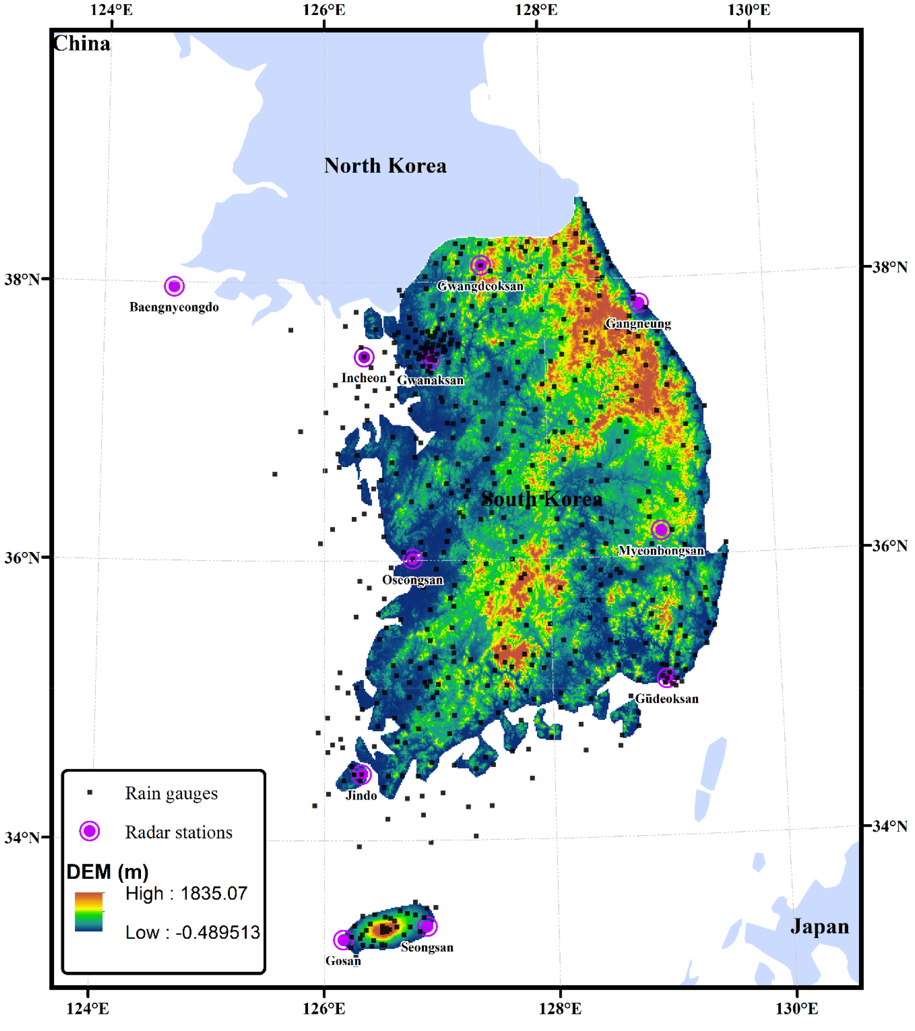
Because these datasets differ in temporal resolution and spatial coverage, a preprocessing workflow was applied to ensure consistency. Ground-based precipitation data were aggregated to 15-minute intervals. Radar reflectivity was converted to rainfall using the Z-R relationship Z=200R1.6 (Marshall and Palmer, 1948) and outliers were removed following Kim et al. (2024). To generate the precipitation field used in the model, radar and gauge observations were combined using the Conditional Merging (CM) technique at 15-minute and 500-meter resolution, as detailed in Section 3 (Ehret, 2003; Sinclair and Pegram, 2005). This approach integrates the spatial continuity of radar with the point-based accuracy of gauges, resulting in a spatially consistent and accurate composite precipitation field.
Temperature and humidity fields were interpolated from station data to the model grid using bi-harmonic spline interpolation, also described in the methodology. These preprocessed gridded meteorological inputs serve as the basis for real-time snow depth simulation across the study domain.
3. Methodology
3.1 Framework overview and real-time workflow
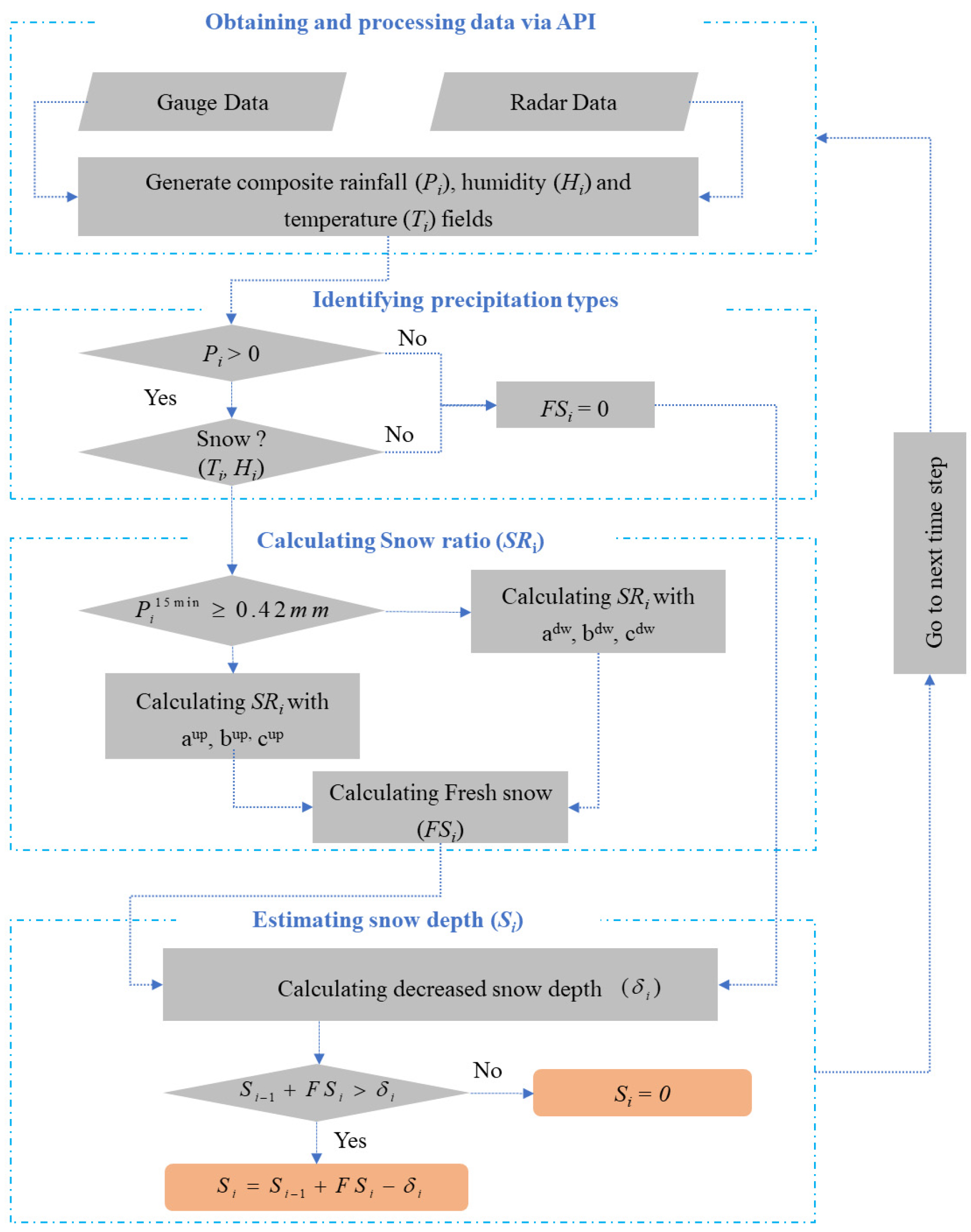
The proposed methodology builds upon the framework of Kim et al. (2025) and is adapted for fully automated, real-time operation. The system consists of five major components: (1) meteorological data acquisition via API from KMA, (2) preprocessing and spatial harmonization of radar and ground data, (3) precipitation phase classification using temperature-humidity thresholds, (4) snow ratio estimation and fresh snowfall calculation, and (5) iterative snow depth updating. Each component operates continuously on a 15-minute basis, enabling dynamic and automated snow monitoring across the study domain (Fig. 2).
3.2 Data acquisition and processing
Meteorological data were collected from two main sources:
Ground-based observations: Precipitation, humidity, temperature and snow from 608 Automatic Weather Stations (AWS) and Automated Synoptic Observing Stations (ASOS) at 15-minute intervals.
Radar observations: Hybrid Surface Rainfall (HSR) data from the Open Radar Product Generator (ORPG) with a resolution of 500 m and 5 minutes.
These datasets were processed to generate composite rainfall (Pi), humidity (Hi), and temperature (Ti) fields. To address differences in temporal resolution radar rainfall were aggregated to 15-minute intervals All variables were then harmonized and resampled to a unified spatiotemporal grid with a resolution of 500 meters and 15 minutes.
These gridded fields, previously introduced in Section 2, serve as meteorological inputs for the snow accumulation and melt modeling framework described in the following sections.
3.3 Precipitation type identification
The classification of precipitation phase in this study follows the shifted Matsuo scheme established by the Korea Meteorological Administration (KMA, 2011) and refined by Lee et al. (2014). This scheme determines precipitation type based on near-surface air temperature T (°C) and relative humidity H (fraction). Five precipitation categories are defined: snow cover (snow accumulation), snow (snowfall), sleet (snow-dominant), sleet (rain-dominant), and rainfall. Among these, snow cover, snow, and sleet (snow-dominant) are considered contributors to snow accumulation and are therefore incorporated into the snow depth simulation framework.
Table 1 summarizes the mathematical thresholds used to classify each type. These thresholds are derived from empirical relationships between temperature and humidity that delineate the phase boundaries for frozen and mixed-phase precipitation. For instance, snowfall can occur at low temperatures and low humidity or at slightly higher temperatures with humidity levels below a dynamic threshold. Rainfall, on the other hand, is identified when RH exceeds a temperature-dependent threshold—typically observed under warmer conditions.
This classification approach offers a practical balance between physical representativeness and computational simplicity and has been validated in operational snow monitoring contexts over South Korea (Park and Kim, 2023). Once snowfall is identified based on the above criteria, the snow ratio (SR) is computed accordingly to estimate fresh snowfall amounts.
At each 15-minute time step, precipitation is first screened (Pi>0) and classified into one of the five types in Table 1 based on temperature (Ti) and humidity (Hi). For the purposes of snow depth modeling, only snow cover, snow, and sleet (snow-dominant) are treated as snowfall indicators. In cases classified as rain, the fresh snowfall (FSi) is set to zero. This conditional filtering, adopted from Kim et al. (2025), ensures the model remains both computationally efficient and physically interpretable under real-time constraints.
Table 1.
Classification criteria for precipitation types based on near-surface temperature and humidity conditions (KMA, 2011; Lee et al., 2014)
| Precipitation type | Calculation |
|
Snow cover (snow accumulation) | ∙ and and |
|
Snow (snowfall) | ∙ and or ∙ and |
| Sleet (snow dominant) | ∙ and and and |
|
Sleet (rain dominant) | ∙ and and or ∙ and |
| Rainfall | ∙ |
At each 15-minute time step, precipitation is first screened (Pi>0) and subsequently classified based on Ti and Hi values into one of the five types described above. If the type is classified as rainfall or sleet (rain-dominant), FSi is set to zero. Otherwise, snowfall proceeds to the SR estimation stage. This classification logic, adopted from Kim et al. (2025) and validated in operational snow monitoring systems (Park and Kim, 2023), ensures a balance between computational efficiency and physical realism—making it suitable for real-time implementation.
3.4 Snow ratio and fresh snowfall estimation
The Snow Ratio (SR) represents the ratio of snowfall depth to precipitation depth and is used to convert liquid-equivalent precipitation into snow accumulation. To reflect the temperature dependency of snowfall processes, this study adopts a sigmoid-shaped nonlinear regression function commonly used in snow hydrology literature (Lee et al., 2005; Byun et al., 2008):
where: Ti is the observed temperature at time step i (°C), and a,b,c are parameters of sigmoid function.
A key advancement in this study lies in the finer temporal resolution of snowfall classification. While Park and Kim (2023) categorized snowfall intensity based on 3-hourly accumulated precipitation, defining light snowfall as events with P < 5 mm/3 h and heavy snowfall as P ≥ 5 mm/3 h, this study translates that classification to a 15-minute interval. Given that 5 mm/3 h corresponds to an average precipitation rate of approximately 0.42 mm per 15 minutes, the same threshold was adopted for consistency. Thus, precipitation events with Pi15 min < 0.42 mm are classified as light snowfall, and those with Pi15 min ≥ 0.42 mm as heavy snowfall. This conversion preserves the empirical basis established in previous research while enhancing the model’s responsiveness to short-term variability. Separate sets of sigmoid parameters are applied for each category to better capture the nonlinear relationship between precipitation intensity and SR at high temporal resolution. This temporal refinement enables faster response to short-lived snowfall events, supporting real-time operational use. The parameters used for SR calculation, as well as those required for melt modeling—including the degree-day coefficient CM, melt correction factor A, and melt threshold temperature T0—were inherited from the optimized results of Kim et al. (2025), as summarized in Table 2. These values were originally calibrated using nationwide data and are adopted here without modification to maintain physical interpretability and numerical stability within a higher-resolution framework.
These parameters, shown in Table 2, were calibrated using eight years of observational data in Kim et al. (2025) and are reused here without re-optimization to enable comparability and operational consistency.
Table 2.
Optimized parameters for snow ratio calculation and melt modeling, adopted from Kim et al. (2025)
| Parameter | P < 0.42 mm/15 mins | P ≥ 0.42 mm/15 mins | |||||||
|
Optimized Value | 12 | 1.4419 | 6.7999 | 8.6250 | 0.5536 | 0.6364 | 0.0024 | 1.97e-02 | -4.7884 |
The amount of fresh snowfall (FSi) at each time step is then calculated as:
To ensure model consistency and operational scalability, a single set of optimized parameters is applied uniformly across the study area. This strategy avoids the need for local calibration and supports real-time deployment using automated API-based input data.
3.5 Snow depth estimation
Following the calculation of fresh snowfall (FSi), the snow depth at each time step Si is updated by accounting for both accumulation and melt processes. The melt rate (Mi) is estimated using the degree-day method, which relates snowmelt to surface temperature. Specifically, melt rate is computed as follows:
where CM is the degree-day coefficient (mm/°C/day), and T0 is the melt threshold temperature (°C). Melt is only considered when Ti > T0; otherwise, Mi = 0. This linear formulation allows for simple and computationally efficient estimation of melt based solely on temperature input.
To account for the influence of snowpack structure on melt dynamics, the actual reduction in snow depth (δi) is calculated by modifying the melt rate with an exponential correction factor that depends on the previous snow depth (Si-1):
where SRx is the snow ratio of the snowpack at position x, A is a melt correction factor (mm-1) that captures nonlinear melt behavior with respect to snowpack size.
Given the lack of detailed observational data on snowpack layering, internal temperature gradients, and snow density evolution due to processes like compaction or refreezing, two simplifications were adopted. First, the SR assigned to each snow event is assumed to remain constant over time. Second, snowmelt is considered to occur only at the surface, progressing sequentially from the top layer downward. These assumptions, validated in the context of Park and Kim (2023), are particularly suitable for real-time applications where high-frequency input data are available, but snowpack stratification data are not.
The updated snow depth is then calculated using:
This formulation prevents negative values and resets the snowpack to zero when complete melting occurs. The entire process operates at a 15-minute temporal resolution and is continuously driven by real-time meteorological inputs retrieved via KMA’s API, allowing the system to dynamically simulate the evolution of snow depth under changing environmental conditions.
4. Results and Discussions
4.1 Model performance evaluation
To evaluate the effectiveness of the proposed snow depth simulation system, a representative snowfall event that occurred between 01 November and 2 December 2024 was selected for detailed analysis. This time window includes multiple snowfall events of varying intensity, offering a robust basis for model evaluation under operational conditions.
The model was executed at a 15-minute temporal resolution and 500-meter spatial resolution, driven entirely by real-time meteorological data retrieved through the KMA API. Input variables—including precipitation, temperature, and humidity—were obtained from 608 automatic weather stations, which were used to generate spatially distributed snow depth estimates across the model domain. However, for model validation, only 94 of these stations provided observed snow depth measurements. Accordingly, the comparison between simulated and observed values was conducted using data from these 94 stations. The simulation results were evaluated using three commonly used performance metrics: the coefficient of determination (R2), root mean square error (RMSE), and Nash-Sutcliffe efficiency (NSE). The following equations were applied.
where Oi and Pi represent the observed and simulated snow depth at time step i, respectively; and are their corresponding means; and n is the number of observation-simulation pairs.
As shown in Fig. 3, the simulation results demonstrate moderate agreement with observed snow depth values, yielding R2 = 0.53, RMSE = 1.03 cm, and NSE = 0.52. These values indicate that the model not only captures the magnitude of snow accumulation accurately but also effectively tracks the temporal evolution of snow depth. The relatively low RMSE reflects minimal absolute deviation from observed values, while the NSE above 0.5 confirms that the model outperforms a simple mean-based predictor.
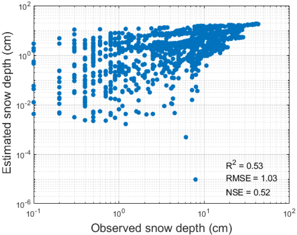
When compared to the radar-based snow depth model developed by Kim et al. (2025)—which reported R2 = 0.71, RMSE = 2.75 cm, and NSE = 0.59 during the validation period of their multi-year experiment (2014-2018) at 1 km spatial and hourly temporal resolution, the proposed model exhibits competitive performance. Despite operating at higher spatiotemporal resolution (500 m × 15 min) and using real-time input data acquired via API, the model achieves an RMSE of 1.03 cm, R2 of 0.53, and NSE of 0.52
Notably, even though our validation period spans only one month, the system successfully simulated maximum snow depths exceeding 43 cm, comparable to the peak values observed during the validation period reported by Kim et al. (2025). The fact that our model maintains significantly lower RMSE under high accumulation conditions highlights its ability to respond to intense snowfall events with high precision. This suggests that real-time processing and finer resolution not only improve responsiveness but also enhance predictive accuracy.
Taken together, these results demonstrate that the proposed real-time system is not only operationally feasible but also statistically robust. The performance gains are particularly relevant for early-warning systems and near real-time applications, where both speed and accuracy are essential.
4.2 Elevation-dependent model performance
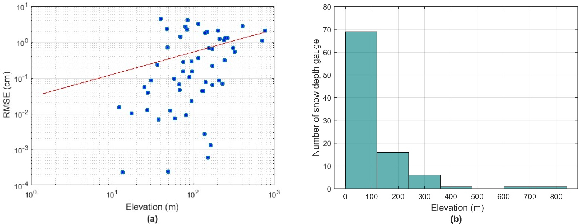
South Korea exhibits highly complex topography, with sharp elevation gradients over short spatial distances due to the presence of major mountain systems such as the Taebaek and Sobaek ranges. Approximately 70% of the national territory is mountainous, leading to significant spatial heterogeneity in meteorological conditions including snowfall intensity, wind exposure, and temperature lapse rates (Kim and Kim, 2013; Hwang et al., 2025). These terrain-induced variations introduce substantial uncertainty in snow depth modeling, particularly when relying on radar-derived precipitation and simplified snow accumulation algorithms. To assess how topography affects model accuracy, the relationship between snow depth estimation error and station elevation was analyzed.
Fig. 4(a) shows the station-wise RMSE plotted against elevation for the 94 snow depth gauges used in this study, with both axes on logarithmic scales. A weak but positive trend is observed, indicating that model errors tend to increase slightly at higher elevations. This elevation-dependent error increase may stem from several physical processes that are more prominent or variable at higher altitudes. For instance, wind-driven snow redistribution can significantly alter snow accumulation patterns, particularly on exposed ridgelines and leeward slopes. Moreover, complex topographic shading, rapid thermal fluctuations, and localized precipitation enhancement due to orographic lifting can all contribute to snowpack heterogeneity. These effects are difficult to capture using uniform snow ratio parameters or temperature-humidity thresholds calibrated primarily for lowland stations. Additionally, the sparse density of observation stations at high elevations limits the availability of ground truth data, which may further hinder the model’s ability to learn or correct biases in complex mountainous terrain. To mitigate model error with elevation, future research could incorporate elevation-based parameter zoning, enabling region-specific tuning of snow ratio and melt parameters. Additionally, the inclusion of terrain-driven variables such as slope, aspect, and wind exposure could further refine snow accumulation estimates. Employing multi-layer snowpack models may also enhance representation of internal snow processes in high-altitude zones. Finally, improving station coverage at higher elevations and integrating cloud-penetrating satellite data such as Sentinel-1 SAR could provide more reliable reference data for validation and calibration.
Fig. 4(b) further reveals that the majority of snow depth stations are located at low elevations, with over 70% situated below 200 meters above sea level. The underrepresentation of high-altitude stations suggests that model performance in mountainous areas may be less constrained by ground truth data, thereby affecting the robustness of validation in complex terrain.
4.3 Validation of snow cover mapping using MODIS NDSI
To evaluate the spatial consistency of the simulated snow depth, this study compared model outputs with satellite-derived snow cover using the Normalized Difference Snow Index (NDSI) from MODIS. NDSI is a widely used spectral index designed to detect snow-covered areas based on the difference in reflectance between visible and shortwave infrared bands. It is calculated as:
where and are surface reflectances in the green (MODIS Band 4) and shortwave infrared (MODIS Band 6) bands, respectively. Snow has high reflectance in the visible spectrum and low reflectance in SWIR, making NDSI an effective indicator of snow cover (Hall et al., 2002).
In this study, the NDSI data were obtained via the Google Earth Engine (GEE) platform using MOD10A1 products, and five cloud-free MODIS images were selected between 1 November and 2 December 2024. Binary snow cover classification was applied to both the MODIS and model outputs for direct comparison. A threshold of NDSI ≥ 0.4 was used to identify snow-covered pixels from MODIS MOD10A1 data. This value is widely adopted in the literature, particularly in mid-latitude regions with complex terrain, where a balance must be struck between sensitivity and specificity (Hall et al., 2002; Zhang et al., 2019). While some studies have proposed adaptive thresholds ranging from 0.3 to 0.45 depending on land cover or atmospheric conditions, a fixed threshold of 0.4 provides a standardized and reproducible basis for large-scale binary classification. Higher thresholds such as 0.5 may lead to underdetection of shallow or mixed-phase snow, particularly in forested or shaded areas where surface reflectance is reduced.
Both the simulated snow depth and MODIS NDSI images were resampled to a common spatial resolution and converted into binary snow presence/absence masks. These were then overlaid to compute pixel-wise classification metrics. The comparison resulted in 151,645 true positives (TP), 150,925 false positives (FP), 154,785 false negatives (FN), and 1,401,000 true negatives (TN). Based on these values, the model achieved an overall accuracy of 0.83, a precision of 0.50, a recall of 0.49, and an F1-score of 0.51.
Although the precision value may appear modest, it reflects well-documented limitations associated with optical satellite-based snow detection, particularly in mountainous regions and during rapidly changing snowfall events. The relatively high number of false positives is likely attributed to a combination of cloud contamination and misclassification in the MODIS NDSI product, underdetection of light or ephemeral snow layers, and temporal discrepancies between the MODIS overpass time and the model’s high-frequency simulation intervals. Notably, the model updates every 15 minutes, potentially detecting short-lived snowfall that has already melted or sublimated by the time MODIS passes overhead. In such cases, the model’s false positives may in fact correspond to real—but temporally mismatched—snowfall events.
Despite these challenges, the balanced F1-score and high overall accuracy indicate a moderate to good agreement between model-simulated and satellite-derived snow cover. Furthermore, the model produces more spatially continuous and topographically coherent snow patterns, which enhances its applicability for real-time snow monitoring. This is particularly beneficial in operational contexts where MODIS observations are frequently hindered by cloud cover or limited temporal resolution.
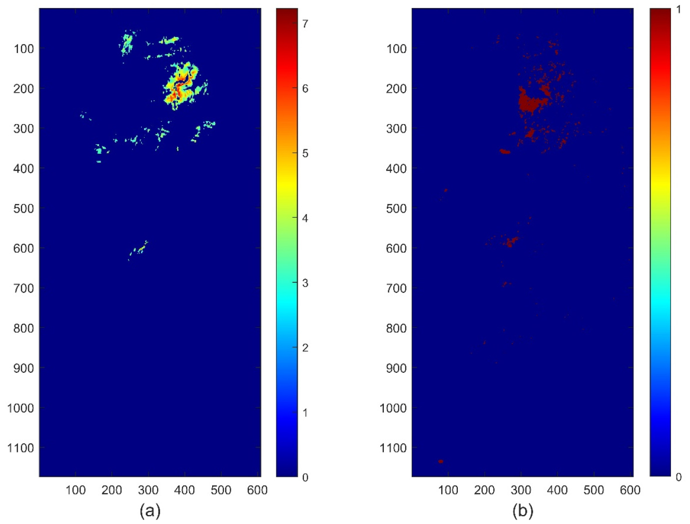
To visually illustrate this agreement, Fig. 5 presents a representative comparison at 10:30 KST on 30 November 2024, a time with widespread snow and minimal cloud cover. Panel (a) displays the simulated snow depth in centimeters from the proposed model, while panel (b) shows the binary snow cover derived from MODIS NDSI using a threshold of 0.4. Both maps consistently detect snow accumulation in the northern part of the study domain. However, the model output reveals a more spatially continuous snow distribution, which can be attributed to the integration of high-resolution radar precipitation and ground-based meteorological observations, offering enhanced spatial coherence compared to satellite-based optical measurements.
Despite the promising performance demonstrated by the proposed system, several limitations remain. First, the model does not explicitly simulate snowpack internal processes such as compaction, refreezing, or layering, which may affect long-term snow water equivalent estimation. Second, cloud cover in MODIS NDSI data limited the number of valid time steps available for spatial validation. This constraint is particularly pronounced during snow events and in mountainous areas where persistent cloud cover can obscure surface conditions. Future efforts could incorporate cloud-penetrating data such as Sentinel-1 SAR or apply data fusion and gap-filling techniques to improve spatiotemporal coverage. Third, the model uses a fixed set of optimized parameters derived from previous research, which may not fully account for regional or seasonal variations in snow dynamics. Future work could address these limitations by incorporating multi-layer snowpack physics, assimilating additional satellite products with higher temporal resolution (e.g., Sentinel-1 SAR), and dynamically adjusting model parameters based on localized ground-truth observations.
5. Conclusion
This study presents a fully automated, real-time snow depth simulation system developed for South Korea, utilizing radar-based precipitation, ground meteorological observations, and physically based threshold modeling. The system operates at 15-minute intervals with a 500-meter spatial resolution, enabling high-frequency, high-resolution monitoring across complex terrain.
Evaluation over the one-month period from 1 November to 2 December 2024 demonstrated strong model performance across multiple snowfall events. Compared to in-situ snow depth observations at 94 stations, the model achieved an RMSE of 1.03 cm, an NSE of 0.52, and an R2 of 0.53—surpassing the accuracy of prior radar-integrated models operating at coarser temporal scales. It also effectively captured high-accumulation events, with maximum depths exceeding 43 cm.
The model showed robust performance across varying elevations, with only a slight increase in RMSE at higher altitudes, likely due to limited station density. Further validation using MODIS-derived NDSI snow cover indicated moderate-to-good spatial agreement, with an overall accuracy of 0.83 and an F1-score of 0.51.
These results underscore the system’s value as a scalable, operational tool for real-time snow monitoring. It holds strong potential for practical applications in early warning systems, winter road management, hydrological forecasting, and disaster risk reduction, especially in data-sparse or topographically complex regions.
Future improvements could include the integration of multi-layer snowpack models, polarimetric radar data, and cloud-penetrating satellite observations such as Sentinel-1 SAR, as well as assimilation of real-time snow sensor networks. These enhancements would further improve model fidelity, especially in high-elevation zones with dynamic snowpack processes. We will also validate the system over at least two additional winters (2024-2026) to assess seasonal robustness.
