

1. 서 론
2. 지배방정식
2.1 유동방정식
2.2 k-ε 난류모형
2.3 경계 조건
2.4 층적분 모형
3. 계산 기법
4. 모의결과
4.1 일반 분포형
4.2 정규화된 분포형
4.3 물 연행
4.4 평형상태의 선단부 속도와 부력 흐름률
4.5 층적분 모형의 형상계수
4.6 층적분 모형과의 비교
4.7
 와
와  의한 영향
의한 영향5. 결 론
1. 서 론
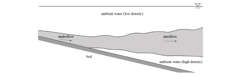
우리나라의 대형 저수지에서는 홍수기에 큰 유량이 발생하여 다량의 부유사가 유입되며, 유입된 부유사는 곧 밀도류의 형태로 전파된다. 밀도류는 주변 수체와의 밀도차에 따라 상층 밀도류(overflow), 중층 밀도류(interflow), 그리고 하층 밀도류(underflow)로 구분된다. 대형 댐의 저수지에서는 유입된 부유사가 Fig. 1과 같이 대부분 하층 밀도류로 시작해 중층 밀도류로 천이되어 전파된다. 중층 밀도류가 발생하는 원인은 저수지의 수체가 온도로 성층화(thermally stratified)되어있기 때문이다. 성층화된 저수지의 하층은 수온이 낮아 수체의 밀도가 높으며, 반대로 상층은 수온이 높아 수체의 밀도가 낮다. 우리나라의 대표적인 대형 댐의 저수지인 소양호의 경우, 여름엔 상층의 수온이 약 27°C까지 상승되는 반면 하층의 수온이 4°C정도로 고정되기 때문에 두 층의 밀도가 약 4 kg/m3정도의 차이를 보인다(Ryu et al., 2011). 따라서 전파되는 밀도류의 밀도가 하층의 밀도보다 높지 않으면, 특정 위치에서 더 이상 하층으로 전파되지 못하고 두 주변수체의 층 사이에서 전파되는 것이다.
중층 밀도류가 하류단에 도달해 제대로 배출되지 않으면 수체의 전반적인 수질 악화를 불러오며, 하층에 태양빛을 차단하기 때문에 다양한 환경적인 문제를 발생시킨다(Chong et al., 2016). 따라서 취수구의 위치를 적절한 위치에 설치해서 상수원에 탁수가 유입되는 것을 방지하거나, 선택적 취수시설(selective withdrawal structure)을 설치해 취수구의 위치를 취수 목적에 따라 조절하기도 한다. 이러한 시설의 설계 및 운영을 효율적으로 하기 위해서는 밀도류의 발달과 전파속도 등의 특성을 이해하는 것이 필수적이다.
과거 하층 밀도류에 대한 연구는 Parker et al. (1987), Altinakar et al. (1990), Garcia (1990), 그리고 Choi and Garcia (1995) 등 많은 연구자들에 의해 수행되었다. 그러나 중층 밀도류에 대한 연구는 하층 밀도류에 대한 연구에 비해 상당히 부족한 상황이다. 중층 밀도류에 대하여 실험을 수행하기 위해서는 하층 밀도류와는 달리 중층 밀도류가 발달되기 위한 성층화된 수체가 필요하다. 그러나 성층화된 수체를 실험수로 규모에서 준비하고 밀도류가 발달되는 동안 유지시키기 어렵기 때문에 얻을 수 있는 자료가 매우 제한적이다. 이로 인해 중층 밀도류의 흐름 구조에 대한 실험 연구사례는 거의 없다.
밀도류의 흐름해석을 위한 수학적 모형은 크게 층적분 모형(layer-averaged model)과 수직구조모형(vertical structure model)으로 나눌 수 있다. Choi and Garcia (1995), Kostic and Parker (2003), Cao et al. (2015), 그리고 Lai et al. (2015)과 같은 많은 연구자들이 층적분 모형을 이용해 실험 수로, 해저협곡, 그리고 댐 상류에서의 부유사 밀도류 전파 및 퇴적에 대해 연구를 수행하였다. 그러나 층적분 모형을 이용해 하층 밀도류 형태로 전파되던 밀도류가 중층 밀도류 형태로 변화하여 전파되는 현상을 모의한 사례는 거의 없다. 층적분 모형을 이용해 중층 밀도류를 계산하기 위해서는 모형에서 사용되는 계수들에 대한 연구가 선행되어야 하지만, 현재까지 중층 밀도류의 모형계수와 관련된 연구는 거의 없다. 실험을 이용해 중층 밀도류의 모형 계수를 얻기는 쉽지 않으므로, 수직구조 모형을 이용하여 얻는 것이 적절하다.
밀도류에 대해 수치모의를 수행할 수 있는 수직구조 모형은 밀도류의 흐름에 대하여 연직방향 분포를 계산할 수 있는 모형이다. 밀도류의 수치모의를 수행하기 위해 주로 난류모형을 이용하여 RANS (Reynolds Averaged Navier-Stokes) 방정식을 해석한다. Stacey and Bowen (1988)은 혼합거리이론을 이용하여 하층 밀도류를 모의하고 Richardson 수에 관계된 하상경사, 바닥항력계수(bottom drag coefficient), 물 연행계수(water entrainment coefficient) 등에 대한 관계를 검토하였고, Choi and Garcia (2002)는  모형을 이용해 하층 밀도류의 수직구조 분포를 분석하고 층 적분 모형에서 사용되는 물 연행계수와 형상계수를 분석하였으며,
  모형의 모형상수를 검토하였다. Ohey and Schleiss (2007)는
  모형을 이용해 투과성 장애물을 설치한 수로에서 밀도류 포집에 대한 효율을 검토하였다. Paik et al. (2009)은 URANS를 이용하여 밀도류의 매우 작은 흐름까지 수치모의를 수행하여 불연속적으로 유입된 밀도류의 전파양상을 재현하였으며 바닥의 경계조건, 벽의 경계조건, 그리고 격자 크기에 따른 모의 결과를 비교하고 분석하였다. 그 외에도 Chung et al. (2009)과 An and Julien (2014)은 수직구조 모형을 이용해 각각 대청호과 임하호에서 발생한 중층 밀도류에 대해 수치모의를 수행하여 선택적 취수시설의 효용성을 검토하였다. 그러나 수직구조 모형을 이용하여 중층 밀도류의 흐름 구조에 대한 분석을 제시한 사례는 없다.
본 연구의 목적은  모형을 이용하여 중층 밀도류의 수직구조에 대해 수치모의를 수행하는 것이다. 이를 위해 밀도류가 전파되는 깊은 수체에
  모형을 적용하여 유속, 초과밀도, 그리고 난류운동에너지의 분포에 대해 분석하였다. 또한 층적분 모형도 같은 수체에 적용하여
  모형의 결과와 비교하였다. 분석한 수치모의 결과를 이용하여 층적분 모형에서 필요한 형상계수를 선정하며 밀도류 계산에서 사용하는
  모형의 모형상수를 검토하였다.
2. 지배방정식
2.1 유동방정식
2차원 RANS 방정식과 초과밀도(excess density) 방정식에 Boussinesq 근사와 경계층 근사(boundary layer approximation)를 적용하면 다음과 같은 Reynolds 평균된 연속방정식,  방향 운동량방정식,
  방향 운동량방정식, 그리고 초과밀도 방정식을 유도할 수 있다.
 (1)
(1)
 (2)
(2)
 (3)
(3)
 (4)
(4)
여기서,  와
와  는 각각 주 흐름방향과 수직방향 위치,
  는 시간,
는 시간,  와
와  는 주 흐름방향과 수직방향 시간평균유속,
  는 시간평균압력,
  는 시간평균초과밀도,
  는 레이놀즈 응력,
  은 난류 스칼라 흐름률, 그리고
  는 중력가속도이다. Eq. (3)을 이용해서 계산된
  를 Eq. (2)에 적용하면 다음과 같이 3개의 식으로 표현된다.
 (5)
(5)
 (6)
(6)
 (7)
(7)
여기서,  는
는  축에서 자유수면까지의 거리다.
2.2  난류모형
난류모형
레이놀즈 평균에 의해 발생한 폐합문제를 해결하기 위해 본 연구에서는 와점성 추정법과  모형을 사용하였다. 레이놀즈 응력과 난류 스칼라 흐름률은 와점성계수를 이용하면 다음과 같이 계산할 수 있다.
 (8)
(8)
 (9)
(9)
여기서,  는 와점성계수,
  는 Prandtl-Schmidt 수이다. 와점성계수는 Prandtl-Kolmogorov 관계식을 통해 다음과 같이 계산한다.
 (10)
(10)
여기서,  는 난류운동에너지,
  는 난류운동에너지의 소산율, 그리고
  는 경험상수다.
  와
와  은 다음의 Eqs. (11) and (12)와 같이 각각의 수송방정식을 이용하여 계산한다.
 (11)
(11)
 (12)
(12)
여기서,  ,
,  ,
,  ,
,  , 그리고
, 그리고  는 경험상수이며
  와
와  는 각각 유속과 부력에 의한 난류생성항이다. 각각의 난류생성항은 Eqs. (13) and (14)를 이용하여 계산한다.
 (13)
(13)
 (14)
(14)
여기서,  는 부피팽창계수(volume expansion coefficient)로 경험상수다. Rodi (1984)는 각각의 경험상수에 대하여
  ,
,  ,
,  ,
,  ,
,  ,
,  , 그리고
, 그리고  을 제시하였다.
  는 부력에 의한 영향을 고려하여 Launder (1975)가 제시한 관계식을 이용하여 계산하였다.
2.3 경계 조건
본 연구에서는 모형의 적용을 위해 Fig. 1과 같이 정지된 주변 수체에서 특정 구간에 밀도류의 유입이 이루어지는 흐름을 모의하였다. 중층 밀도류가 중앙선을 기준으로 대칭된 형태를 보인다고 가정하고 상층만을 계산구역으로 설정하였다. 유입부의 경계조건은 아래와 같이 설정하였다.
 (15)
(15)
 (16)
(16)
 (17)
(17)
 (18)
(18)
여기서,  ,
,  ,
,  , 그리고
, 그리고  는 각각 유입부에서의 최대값이고
  는 유입된 밀도류의 두께로 Table 1에 제시하였다. 유입부의 밀도 Froude 수
  는 6.06으로 supercritical flow다.
  와
와  는 Ferziger and Peric (1996)이 제시한 값,
  과
과  을 사용하였다. 상층과 하층의 경계면은
  방향으로 변화율이 0인 조건(
 )을 사용하였고, 유출부의 경계면은
  방향으로 충분히 발달되어 변화율이 0인 조건(
 )을 사용하였다.
  는 유출부를 제외한 모든 경계면에서 0을 사용하였다.

2.4 층적분 모형
Eqs. (5)~(7)을 밀도류의 중앙부에서 자유수면까지 층적분하면 다음과 같이 중층 밀도류에 대한 층적분된 식을 얻을 수 있다.
 (19)
(19)
 (20)
(20)
 (21)
(21)
여기서,  는 층적분된 밀도류의 두께,
  는 층적분된 유속,
  는 층적분된 초과밀도,
  는 형상계수이다.
  는 물 연행계수로서 Parker et al. (1987)은 다음과 같은 관계식을 제시하였다.
 (22)
(22)
여기서,  는 Richardson 수(
 )다.
)다.
3. 계산 기법
밀도류는 강한 이류성 흐름이므로 Eqs. (5)~(7), (11) and (12)를 수치해석하기 위해 이송항에 대하여 UPWIND 기법을 사용하였으며, 시간항에 대해서 explicit 기법을 사용해 계산하였다. 각 방향 계산격자의 크기, 계산격자의 수, 그리고 CFL 수는 Table 2에 제시하였다. 층적분 모형은 이동경계조건을 사용하고 ULTIMATE-QUIKCKEST 기법을 사용하여 계산하였다. 층적분 모형에 대한 검증은 Choi and Choi (2017)에서 수행하였으므로 본 연구에서는 검증을 위한 계산은 수행하지 않았다.

4. 모의결과
4.1 일반 분포형
Fig. 2는 밀도류가 발생하는 영역에서 유속과 초과밀도분포를 도시한 것이다. 밀도류가 주 흐름방향으로 진행하면서 연직방향으로 점점 확산되고 유속과 초과밀도가 점점 감소하는 것을 알 수 있다. 또한 밀도류가 확산되면서 유속과 초과밀도의  방향 변화율이 감소되는 것을 볼 수 있다. 유속과 초과밀도류의
  방향 변화율이 감소되면 와점성 추정법을 사용하는
  모형에 의해 운동량과 초과밀도의
  방향 교환 역시 감소되어 주 흐름방향에 따른 밀도류의 연직방향 확산률이 점점 작아지게 된다.

4.2 정규화된 분포형
Figs. 3(a)~3(d)의  축은 각각 주 흐름방향 유속, 초과밀도, 난류운동에너지, 그리고 난류운동에너지의 소산율을 나타내며, 각각의 값을 층적분된 값(
 ,
,  ,
,  , 그리고
, 그리고  )으로 무차원화 한 것이다.
  축은 수직방향 위치를 층적분된 두께(
 )로 무차원화 하였다. 점선은 같은 초기 두께, 유속 조건에서 하층 밀도류일 때의 값이다. Fig. 3을 통해 밀도류의 수직구조에 관한 유사성(similarity collapse)을 확인할 수 있다. Fig. 3을 보면 유속과 초과밀도는 밀도류 중앙에서 최대점을 갖지만, 난류운동에너지와 난류운동에너지의 소산율은
  지점에서 최대점을 가지고 밀도류의 중앙에서 매우 작은 것을 볼 수 있다. 난류운동에너지와 그 소산율이 밀도류 중앙에서 작은 값을 가지는 이유는 와점성개념을 사용하는 난류모형의 한계로 보인다.
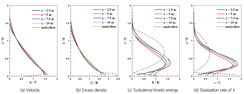
Fig. 3에서 유속이나 초과밀도는 각 위치에 따른 유사성을 보인다. 그러나 난류운동에너지와 그 소산율은 밀도류 중앙에서 주 흐름방향으로 갈수록 크게 감소되기 때문에 적분된 값인  와
와  도 작게 산정된다. 따라서 Figs. 3(c) and 3(d)는
  와
와  로 무차원화 하면서
  지점에서
지점에서  와
와  이 주 흐름방향으로 갈수록 큰 값으로 보여 유사성이 약한 것처럼 보이는 현상이 발생한다. 중층 밀도류의 초과밀도의 경우 하층 밀도류의 초과밀도와 분포 형태가 거의 비슷하며 바닥 근처에서만 약간의 차이를 보인다. 이것을 통해 중층 밀도류의 형상계수
  과
과  가 하층 밀도류의 형상계수와 비슷할 것임을 예상할 수 있다.
4.3 물 연행
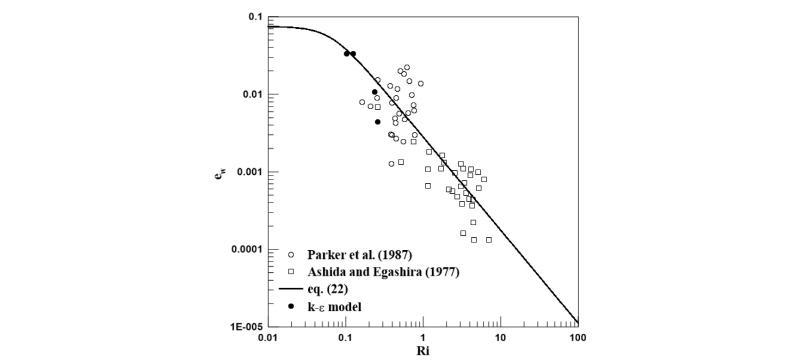
Fig. 4는 물 연행계수  를 계산하여 기존의 실험 결과와 Parker et al. (1987)이 제시한 경험식과 비교한 것이다.
  는
는  모형을 이용하여 계산된 결과를 층적분한 다음, 층적분 모형인 Eq. (19)에 두께와 유속 자료를 적용하여 역계산하였다. 물 연행계수는 기존 연구와 같이 Richardson 수에 반비례하는 관계를 보이며 Parker et al. (1987)이 제시한 경험식과 잘 맞는 것을 볼 수 있다. 이를 통해 중층 밀도류의 물 연행에 대해서는 하층 밀도류에서 사용하는 물 연행계수를 동일하게 사용할 수 있을 것으로 판단된다. 그러나 충분히 발달된 영역에서 물 연행계수가 크게 감소하는 것을 볼 수 있다.
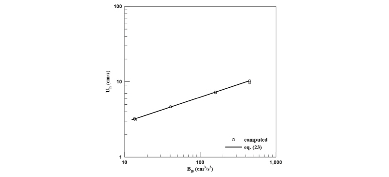
4.4 평형상태의 선단부 속도와 부력 흐름률
밀도류는 지속적인 물의 연행에 의해 밀도류의 두께가 증가하게 된다. 따라서 밀도류는 유속이 일정할 때 Richardson 수가 일정하게 된다. 이 때 동일한 두께증가율을 가지며, 이를 평형상태로 본다. 평형상태가 되었을 때 유속과 Richardson 수를 각각 평형 유속과 평형 Richardson 수라 부른다. Fig. 5는 평형상태일 때의 선단부 속도(head velocity)와 부력 흐름률(Buoyancy flux)의 관계를 도시한 것이다. 이를 위해 유입부의 두께, 속도, 초과밀도 등을 변화시켜가며 비교해 보았다. 계산 결과 중층 밀도류의 선단부 속도는 부력 흐름률의 3제곱에 비례하는 것을 볼 수 있다.  = 1.33으로, 이것은 Britter and Linden (1980)가 제시한 하층 밀도류에서 선단부 속도와 부력흐름률에 대한 관계식과 거의 유사하며, 그 식은 다음과 같다.
 for
for (23)
(23)
여기서,  는 하상의 경사이다.
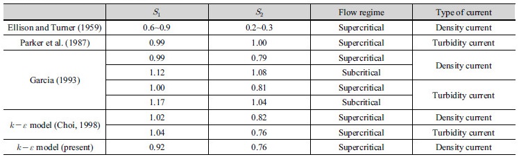
4.5 층적분 모형의 형상계수
층적분 모형을 중층 밀도류에서 계산하기 위해서는, 모형에서 사용되는 형상계수를 계산할 필요가 있다. 따라서  모형을 이용해 계산된 초과밀도분포를 다음과 같이 적분하였다.
 (24)
(24)
 (25)
(25)
여기서,  는
는  다. Table 3은 기존 연구자들이 제시한 형상계수와 본 연구에서 계산된 형상계수를 비교한 것이다.
  은 0.92로 이는 다른 연구자들의 계산결과와 마찬가지로 1에 가까운 값이 계산되었고,
  는 0.76으로 상대적으로 약간 작은 값이 계산되었다. 중층 밀도류와 하층 밀도류의 형상계수가 매우 유사한 값을 가지는 것을 수 있는데, 그 이유는 중층 밀도류의 초과밀도분포가 하층 밀도류의 형태와 유사하기 때문이다.
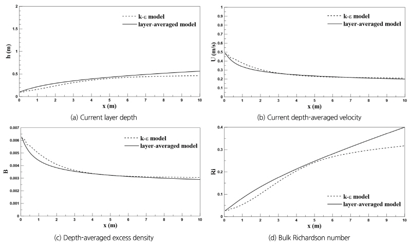
4.6 층적분 모형과의 비교
Fig. 6은  방향으로 발달하는 중층 밀도류를 도시한 것이다. 그림에서
  모형에 의한 결과와 층적분 모형에 의한 결과를 함께 제시하였다.
  모형의 결과를 층적분하기 위해 다음과 같은 식을 사용하였다.
 (26)
(26)
 (27)
(27)
 (28)
(28)
층적분 모형에서 물 연행계수는 Eq. (22)의 것을 사용하였고, 형상계수는 4.5 층적분 모형의 형상계수에서 제시한 값을 사용하였다. Fig. 6(a)에서  모형을 이용해 계산된 밀도류의 두께가 층적분에 의해 계산된 것 보다 조금 더 작은 것으로 계산된다.
  모형은 초기 경계조건에서 설정된 유속분포형에서 시작되기 때문에 유속분포에 의해 계산된 두께가 다른 지점에 비해 작은 값을 가진다. Fig. 3(a)를 보면
  일 때 유속이 분포하는 최대
  가 다른 지점에 비해 높은 것으로
  가 작게 산정된 것을 예상할 수 있다. 반면 층적분 모형은 수직 구조의 유사성을 가정한 모형이기 때문에 유속분포를 일정하게 예상하고 계산하므로 유입부 근처에서
  모형과 밀도류 두께의 차이를 발생시킨다. 또한, 4.3 물 연행에서
  모형이 높은 Richardson 수에서 물 연행을 작게 산정하는 것을 보였다. Fig. 6(d)에서 주 흐름방향으로 진행되면서 Richardson 수가 증가되는 것을 볼 때
  모형이
모형이  지점부터 층적분 모형의 물 연행에 비해 적게 물을 연행하여 두 모형의 두께 차이가 발생하는 것을 알 수 있다. Figs. 6(b) and 6(c)를 보면 유입부 근처에서 수직 구조의 유사성의 문제로
  모형이 층적분 모형에 비해 유속과 초과밀도를 크게 계산하지만 그 이후부터는 거의 일치하는 것을 볼 수 있다.
 model and layer-averaged model
4.7 와 에 의한 영향
Eqs. (10)~(12)의 경험상수들은 많은 연구자들에 의해 제시가 되었으나, 무차원 부피팽창계수  와 경험상수
  는 아직 확실한 값이 제시되지 않았다. Fukushima and Hayakawa (1990)은
  이 0~0.4의 범위에 있을 경우 수치해와 실험결과가 잘 맞는 것을 보였고, Choi and Garcia (2002)는 하층 밀도류에 대해
  = 0.29일 때
  모형과 층적분 모형이 일치함을 밝혔다. 그 외에도 Gibson and Launder (1976)은
  = 0을, Svensson (1980)은
  = 0.6을, 그리고 Hossain and Rodi (1982)는
  = 1을 제시하는 등 많은 연구자들이 서로 다른 대상에 따라 다른
  값을 제시하였다. 중층밀도류에
  에 대한 적합한 값이 제시된 바가 없으므로 중층 밀도류에 적합한
  값과
값과  를 확인해 볼 필요가 있다.
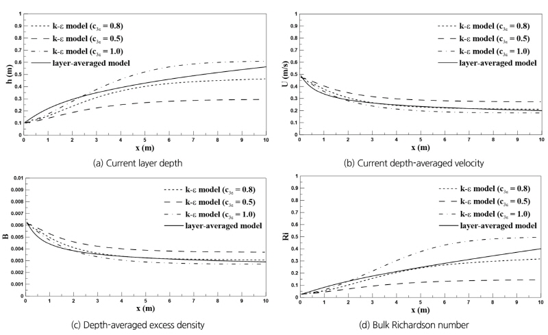
Fig. 7은  를 10으로 고정하고
  이 0.5, 0.8, 그리고 1.0일 때
  모형을 적용한 결과와 층적분 모형의 결과를 비교한 것이다. 그림을 보면
  가 클수록
가 클수록  모형이 밀도류의 두께를 크게 산정하고 유속과 초과밀도를 작게 산정하는 것을 볼 수 있다. 이것은 Eq. (12)의 난류생성항
  가 음의 값을 가지기 때문이며, 난류운동에너지의 소산율을 감소시켜 난류에 의한 물 연행을 더 증대시키기 때문이다. 층적분 모형과 비교한 결과
  모형이
모형이  을 0.8~1.0의 값을 사용하였을 때 밀도류의 두께를 유사하게 모의하는 것을 볼 수 있다. 그리고
  모형이
모형이  을 0.8의 값을 사용하였을 때 밀도류의 유속과 초과밀도를 가장 잘 모의하는 것을 보인다.
 on
on  model (
 )
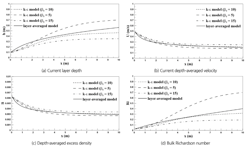
)Fig. 8은  을 0.8로 고정하고
  를 5, 10, 그리고 15를 사용할 때
  모형의 결과와 층적분모형의 결과를 비교한 것이다. 그림을 보면
  가 클수록
가 클수록  모형이 밀도류의 두께를 작게 산정하고 유속과 초과밀도를 크게 산정하는 것을 볼 수 있다. 이것은 난류생성항
  가 음의 값을 가져 난류운동에너지를 감소시켜 난류에 의한 밀도류의 물 연행을 감소시키며,
  를 증가시켜 초과밀도의 연직방향 확산을 감소시키기 때문이다. 층적분 모형과 비교 결과
  = 10일 때 가장 잘 맞는 결과를 보이며, 이는 Rodi (1984)가 제시한 값과 일치한다.
 on
on  model (
 )
)5. 결 론
본 연구에서는  모형을 이용하여 중층 밀도류에 관한 수치모의를 수행하였다. 수치모의를 통해 깊은 수체 내부에서 발달된 밀도류의 유속, 초과밀도, 난류운동에너지에 대해 분석하였다. 또한 층적분 모형에 사용되는 형상계수와 밀도류의 특성에 대하여 분석하였으며, 여러 논문에서 다른 값을 제시하는
  모형의 모형상수에 대해서도 분석하였다.
 모형이 중층 밀도류가 하류 방향으로 전파되면서 연직방향으로 확산되고 유속이 감소하며, 연직방향 확산률이 점차 감소되는 것을 모의하였다. 밀도류의 유속이나 초과밀도에 대하여 층적분된 값으로 수직구조를 비교해보면 유사성을 보이며, z = 0 근처 지점을 제외하면 하층 밀도류와 매우 유사한 것을 확인할 수 있다. 난류운동에너지와 그 소산율은 밀도류의 중앙에서 크기가 점점 작아지는 영향으로 유사성이 약하게 보인다.
하층밀도류에서 사용하는 물 연행계수를 이용해 중층 밀도류의 물 연행에 대하여 검토하였다. 그리고 밀도류가 평형상태일 때 선단부의 속도는 부력흐름률의 1/3제곱에 비례하는데 이것은 Britter and Linden (1980)이 제시한 하층 밀도류에 대한 관계식과 유사한 것을 확인하였다. 또한 층적분 모형에서 사용하는 중층 밀도류의 형상계수를 계산해본 결과, 하층 밀도류에서 사용하는 값과 큰 차이가 없는 0.76인 것을 검토하였다.
 과
과  를 검토하기 위해
  모형의 결과를 층적분한 값과 층적분 모형의 결과를 비교하였다.
  과
과  가 부력에 의한 난류생성을 조절하며
  는 또한 초과밀도의 확산을 직접 조절하기 때문에 밀도류의 두께를 조절하는 것을 확인하였다.
  과
과  에 대하여 중층 밀도류에 가장 적합한 값은 Rodi (1984)가 제시한
  = 0.8과
  = 10인 것을 검토하였다.
