

1. 서 론
2. 기본 이론
2.1 교차상관분석
3. 연구 방법 및 자료
3.1 연구 방법
3.2 연구자료
3.2.1 강수 및 기온자료
3.2.2 기상인자 자료
4. 연구 결과
4.1 강수와 기상인자간의 상관관계
4.2 기온과 기상인자간의 상관관계
5. 결 론
1. 서 론
강수 및 기온은 일상생활과 밀접하게 관련되어 있어 방송 등의 매체를 통해 이러한 기상현상들에 대한 단기/장기 예보를 실시하고 있다. 하지만 이러한 예측이 항상 정확히 일치하지 않으며 종종 잘못된 예보로 인해 피해가 발생하고 있다. 따라서 이러한 기상현상에 대한 예측은 매우 중요한 연구 중에 하나로 꾸준히 진행되어 왔으며, 최근 기후변화로 인한 기상이변이 빈번히 발생하면서 좀 더 정확한 강수 및 기온의 예측의 필요성이 증대됨에 따라 다양한 방법을 통해 예측의 정확도를 높이려는 연구가 꾸준히 진행되고 있다.
그 중 기상현상의 장기적인 예측을 위해 기상인자를 통한 대규모 기후변동과 강수 및 기온간의 상관성 분석을 통해 장기적인 예측의 정확도를 높이려는 연구도 활발히 진행되고 있다. 대규모 기상변동과 기상현상과의 상관성을 분석하기 위해 대규모 기상변동을 수치화 할 수 있는 다양한 기상인자가 개발되어 왔는데, Walker and Bliss (1932)는 NAO (North Atlantic Oscillation), NPO (North Pacific Oscillation) 등의 기상인자를 개발하여 북반구에서의 대규모 대기순환을 통해 기온 및 강수 등의 기상활동에 대한 예측을 수행하였다. Wallace and Gutzler (1981)는 500 mb 고도장과 해면기압도를 이용해 겨울철 북반구에서의 대기 움직임을 분석하였으며 그 결과 북반구 내에서는 해면기압의 분포가 위도별로 대칭적인 분포를 가지며, 이러한 패턴은 중대류권(mid-tropospheric)에서 더욱 뚜렷하게 나타나는 것을 발견했다. 이러한 텔레커넥션 패턴을 통해 겨울철 북반구 기상현상의 예측 인자로 활용성이 있는 WP (Western Pacific pattern), PNA (Pacific North American pattern)를 개발하였다. Rasmusson and Carpenter (1982)는 엘니뇨 남방진동의 변동성을 살펴보기 위해 엘니뇨 지역(적도 태평양)을 1, 2, 3, 4 등의 지역으로 구분하여 해수면온도, 바람장, 해면기압 등의 요소로 분석하고 그 변동성을 살펴보았다. Ropelewski and Jones (1987)는 남방진동의 변동을 지수화하기 위하여 남태평양 Tahiti와 Darwin 지역의 해면기압 차를 SOI (Southern Oscillation Index)로 제시하고 엘니뇨 남방진동과의 관련성을 분석하였다. Wolter and Timlin (1993)은 기상인자를 이용한 엘니뇨 분석의 정확도를 높이기 위해 기존의 특정 기상요소를 고려한 분석과는 다르게 해면기압(Sea Level Pressure, SLP), 해수면온도(Sea Surface Temperature, SST), 위도간 표면 바람장(zonal surface wind), 경도간 표면 바람장(zonal meridional wind), 표면대기온도(surface air temperature), 총 운량(total cloudiness)등 6개 요소의 주성분분석(Principal Component Analysis, PCA)을 통해 MEI (Multi-variative ENSO Index)를 제시하여 엘니뇨의 변동성을 분석하였다. Mantua et al. (1997)은 태평양 해수면 온도의 주성분분석을 통해 개발한 PDO (Pacific Decadal Oscillation)와 태평양 해수면온도 간의 상관관계를 통해 엘니뇨와 PDO 사이에 관련성이 있음을 밝혔고 그로 인한 영향을 분석하였다. Thompson and Wallace (1998)는 북극 지역의 1000 mb 고도장의 첫 번째 EOF (Empirical Orthogonal Function)를 지수화한 AO (Arctic Oscillation)를 제시하여 기존의 NAO보다 좀 더 정확하게 겨울철 북반구 유라시아 지역의 해면기압장의 순환을 설명하였다.
또한 이러한 기상인자들을 통해서 강수 및 기온간의 상관관계를 분석한 연구가 진행되어 왔는데, Ropelewski and Halpert (1987)는 태평양에서의 강수가 엘니뇨에 직접적인 영향이 있음을 밝히고, 태평양 주변의 호주, 북아메리카, 남아메리카, 인도 남부, 아프리카 등에서의 계절별 변동 특성을 분석하여 엘니뇨로 인한 영향을 설명하였다. Baldwin and Dunkerton (1999)은 AO 패턴과 북반구에서의 10, 30, 50, 100, 200, 300, 500, 700, 1000 mb 고도장간의 패턴 변화 비교, 위도간 평균 바람장, 평균온도 등과의 패턴변화 분석 및 교차상관관계 분석을 통해 AO가 북반구 기온변동에 미치는 영향을 분석하였으며, Terenberth et al. (2000)은 ENSO가 북태평양-북아메리카 지역의 강수와 비선형적인 연관성을 가지고 있다고 밝히고, 적도 부근의 해수면 온도를 warm phase/cold phase로 나누어 그 역학적인 관계를 분석하였다. Higgins et al. (2000)은 겨울철 미국의 기온 변화를 AO와 ENSO (El-Nińo Southern Oscillation)의 상관성을 중심으로 분석하였으며, Larson et al. (2005)은 엘니뇨와 AO를 통해 미국-멕시코 지역의 사이클론 발생과의 상관성을 200 mb 고도장/바람장을 이용하여 분석하였다. Lee and Ouarda (2013)는 경험적 모드분해법을 통해 PDO와 NAO를 분석하고 그 상관관계를 찾아 태평양과 대서양에서의 기후변동의 관련성을 분석하였다.
본 연구에서는 기상인자와 우리나라 강수 및 기온과의 상관성을 분석하는 데에 있어서 원 자료간의 상관관계가 아닌 경험적 모드분해법을 이용해 분해한 강수 및 기온자료를 바탕으로 기상인자와의 상관성을 주기성과 경향성에 따라 분석하여 좀 더 명확한 상관관계를 도출하였다. 이를 통해 우리나라 기상활동과 연관이 있는 대규모 기후변동을 찾고, 이를 통해 상관관계가 나타난 기상인자를 강수 및 기온의 장기적인 예측을 위한 인자로의 활용 가능성을 살펴보았다.
2. 기본 이론
2.1 교차상관분석
교차상관분석은 신호처리의 한 분야로서, 두 시계열중 하나에 시간차(lag)를 두어 두 자료계열의 유사성을 측정하는 방법이다. 동일한 자료 기간을 갖는 두 시계열 자료  ,
,  (
( )에 대해
)에 대해  만큼의 시간차를 갖는 교차공분산
  는 Eq. (1)과 같이 구한다.
 ,
,  (1)
(1)
여기서  ,
,  는 각 자료계열의 평균을 의미한다.
Eq. (1)에서 구한  를 Eq. (2)와 같이 각 자료계열의 표준편차로 나눈 결과가 교차 상관계수가 되며, 상관계수가 +1인 경우는 두 자료가 완전히 일치하는 것을 의미하고 –1인 경우는 완전히 반대의 위상을 갖는 것을 의미하며 그 값이 0에 가까울수록 두 자료의 상관관계는 없는 것을 의미한다(Box et al., 1994).
 (2)
(2)
3. 연구 방법 및 자료
3.1 연구 방법
우리나라 강수 및 기온자료와 기상인자와의 상관관계 분석을 위해 앞선 “경험적 모드분해법을 이용한 기상인자와 우리나라 강수 및 기온의 상관관계 분석 : I. 자료의 분해 및 특성분석” 연구를 통해 추출한 강수 및 기온자료를 대상으로 기상인자와의 상관관계 분석을 수행하여 좀 더 명확하고 구체적인 관계를 도출하고자 하였다. 선별된 강수 및 기온의 내재모드함수를 기상인자와의 교차상관관계 분석을 통해 상관계수가 높게 나타난 기상인자들을 선별하고, 선별된 기상인자가 갖는 의미를 통해 우리나라 기상현상에 영향을 미치는 대규모 기후변동을 찾아 우리나라 기상의 장기예측에 대한 활용성을 검토하였다.
3.2 연구자료
3.2.1 강수 및 기온자료
기상인자와의 상관관계 분석을 위한 강수 및 기온자료는 앞선 연구에서 수행한 우리나라 기상청 14개 지점 월강수총량, 월평균기온의 내재모드함수 중 유의성 검정을 통해 선별된 자료를 시용하였다. 지점은 1960년부터의 2014년까지 660개월의 자료기간을 가지며 Table 1은 대상 지점에서의 자료기간 및 선별된 내재모드함수를 나타내었다.
 s
s ,
,  ,
, 
 ,
,  ,
, 
 ,
,  ,
, 
 ,
,  ,
, 
 ,
,  ,
, 
 ,
,  ,
, 
 ,
,  ,
, 
 ,
,  ,,
,, 
 ,
,  ,
, 
 ,
,  ,
, 
 ,
,  ,
, 
 ,
,  ,
, 
 ,
,  ,
, 
 ,
,  ,
, 
 ,
,  ,
, 
 ,
,  ,
, 
 ,
,  ,
, 
 ,
,  ,
, 
 ,
,  ,
, 
 ,
,  ,
, 
 ,
,  ,
,  ,
, 
 ,
,  ,
, 
 ,
,  ,
, 
 ,
,  ,
, 
 ,
,  ,
, 
 ,
,  ,
, 
 ,
,  ,
,  ,
, 
 ,
,  ,
, 
3.2.2 기상인자 자료
강수 및 기온 자료와 상관관계를 분석하기 위한 기상인자 자료로 NOAA ESRL (Earth System Research Laboratory)에서 제공하는 39개 기상인자 자료를 사용하였다. 기상인자는 크게 해수면 온도 관련 인자, 대기운동 관련인자, 강수 및 기온 관련인자, 복합 인자 등 4가지로 분류되며 Table 2에서 39개 기상인자 자료의 명칭, 관측기간 등을 정리하였다.
4. 연구 결과
4.1 강수와 기상인자간의 상관관계
교차상관계수를 통한 강수량과 기상인자간의 상관관계 분석 결과 주기성과 경향성 모두 상관관계를 확인할 수 있었다. 강수량 시계열의 주기성을 설명할 수 있는  에서 엘니뇨 및 강수와 연관된 기상인자와 높은 상관관계를 보였으며, 해수면온도 또는 기온과 관련된 기상인자에서 경향성을 나타내는
  과의 상관관계가 높게 나타났다. 다음의 Table 3은 14개 지점의 강수자료와의 상관관계 분석 결과 중 유의할 만한 상관관계를 보이는 기상인자와 그 때의 시간차를 정리한 결과이다.
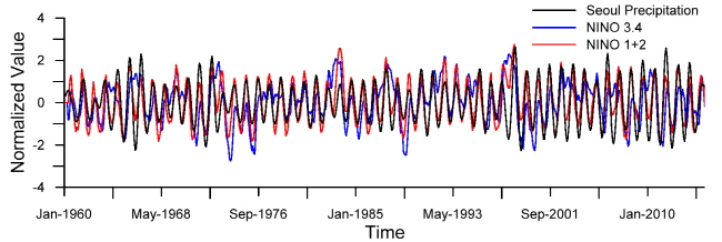
엘니뇨 현상과 관련하여 NINO 1+2 지역의 해수면 온도와의 상관계수는 대부분의 지점의  에서 4개월의 시간차를 두고 0.7에 가까운 높은 상관계수를 보였다. 또한 NINO 3.4, NINO 3 지역의 해수면 온도와는 대부분 지점의
  에서 3개월의 시간차를 두고 0.3 이상의 상관계수를 나타내었다. 이는 엘니뇨 현상과 깊은 관련이 있는 적도 태평양의 해수면온도, 특히 엘니뇨 현상에 가장 민감한 온도 변화를 보이는 NINO 1+2 지역과 큰 상관계수를 가진다는 것은 우리나라의 강수 패턴이 엘니뇨 현상과 깊은 관련이 있음을 의미한다. Fig. 1은 서울 지점 강수의
  와 4개월의 시간차 만큼 이동한 NINO 1+2 지역 해수면 온도 시계열과, 3개월의 시간차 만큼 이동한 NINO 3.4 지역의 해수면 온도 시계열을 각 자료계열의 평균과 분산을 이용하여 정규화시킨 자료를 도시한 그림이다. 이를 통해 세 시계열간의 주기가 일치하며 비슷한 패턴으로 시계열이 증감함을 도시적으로 확인할 수 있다.
강수와 관련한 기상인자 중 인도 중부 지역의 강수와 관련된 Central Indian Precipitation의 상관관계 분석 결과 대부분의 지점에서 시간차를 두지 않고 0.5 이상의 높은 상관관계를 보였으며, 미국 남서부 내륙지방의 강수와 관련된 SW Monsoon Region rainfall과의 상관관계 분석 결과 대부분의 지점에서 시간차 없이 0.3 이상의 상관계수를 나타내었다. 이는 우리나라의 강수 패턴이 미국 남서부 내륙지방, 인도 중부지방과 유사하다는 것을 보여준다. Fig. 2는 1981년부터 1999년까지 서울 지점 강수의  와 Central Indian Precipitation, SW Monsoon Region rainfall의 정규화된 시계열을 도시한 자료이다. 이를 통해 여름철에 집중되어 많은 강우가 내리고 겨울철에 적은 강우가 내리는 우리나라의 강수 패턴과 두 기상인자간의 유사성을 확인할 수 있다.
추세를 의미하는 잔여요소(residual)와 대서양 해수면 온도와 관련된 AMO, Atlantic Tripole SST EOF, Caribbean Index, NTA, TSA, TNA 및 태평양 해수면 온도와 관련된 WHWP, Pacific Warmpool간의 상관계수는 시간차를 두지 않고 대체로 0.3 이상의 유의할 만한 상관계수를 나타내었다. 또한 전지구적인 기온변화를 나타내는 GMT와는 매우 높은 0.8 이상의 상관계수를 나타내었다. 이는 지구온난화로 인한 해수면, 기온상승의 추세가 우리나라 강수량에도 영향을 미치고 있음을 의미한다. 다음의 Fig. 3은 서울지점에서의 월 강수총량의 잔여요소와 AMO, WHWP, GMT의 시계열을 도시한 그림이다. 그림에서 표시된 굵은 선은 각 기상인자의 6차 다항 회귀식으로 각 기상인자의 변화양상을 파악할 수 있다.
이를 통해 강수 자료의 잔여요소는 점점 증가하는 추세를 보이며, 기상인자의 시계열에서도 마찬가지로 증가하는 추세를 보여 두 계열간의 추세가 일치하는 것을 확인할 수 있으며, 특히 최근들어 그 상승폭이 점점 증가하는 형태를 지닌 GMT와 서울 지점과의 상관관계는 상당히 유사한 면을 보인다.
 (-4)
(-4) (-3)
(-3) (-3)
(-3) (0)
(0) (0)
(0) (0)
(0) (0)
(0) (0)
(0) (0)
(0) (0)
(0) (0)
(0) (0)
(0) (0)
(0) (0)
(0)
|
Fig. 1. Time series of |
|
Fig. 2. Time series of |
 , NINO 1+2, and NINO 3.4 (Precipitation, Seoul)
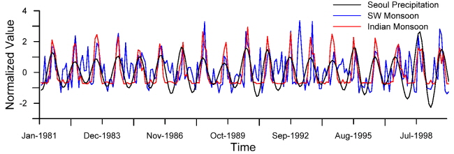
 , SW Monsoon, and Indian Monsoon (Precipitation, Seoul)
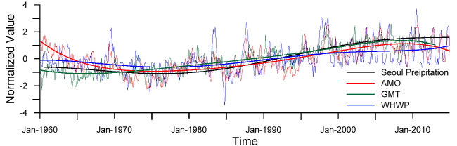
 , AMO, WHWP, and GMT (Precipitation, Seoul)
 (-4)
(-4) (-3)
(-3) (-3)
(-3) (-10)
(-10) (0)
(0) (0)
(0) (0)
(0) (0)
(0) (0)
(0) (0)
(0) (0)
(0) (0)
(0) (0)
(0)4.2 기온과 기상인자간의 상관관계
교차상관계수를 통한 월평균기온과 기상인자간의 상관관계 분석 결과에서도 주기성과 경향성 두 가지 모두의 경우에서 상관관계를 확인할 수 있었다. 주기성과 관련해서  에서 엘니뇨와 연관된 기상인자와 높은 상관관계를 보였으며,
  에서 적도 지역의 성층권에서의 바람장을 나타내는 QBO와 음의 상관관계를 보였다. 추세와 관련해서는 강수량과의 상관관계 분석과 마찬가지로 해수면온도 또는 기온과 관련된 기상인자에서 높은 상관관계를 보였다. 다음의 Table 4는 14개 지점의 기온자료와의 상관관계 분석 결과 중 유의할 만한 상관관계를 보이는 기상인자와 시간차를 정리한 결과이다.
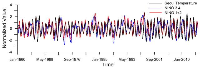
엘니뇨 현상과 관련하여 NINO 1+2 지역의 해수면 온도와의 상관계수는 대부분 지점의  에서 4개월의 시간차를 두고 대체로 0.7이 넘는 상관계수를 보였고, 특히 서울, 부산, 제주 세 지점에서는 0.8이 넘는 높은 상관계수를 보였다. 또한 NINO 3.4 지역의 해수면 온도와는 0.4 이상, NINO 3 지역의 해수면 온도와는 0.6 이상의 유의미한 상관관계를 나타내었다. 이는 강수와 마찬가지로 우리나라 기온의 변화 패턴 또한 엘니뇨 현상과 깊은 관련이 있음을 의미한다. 다음의 Fig. 4는 서울 지점 기온의
  와 4개월의 시간차 만큼 이동한 NINO 1+2, 3개월의 시간차만큼 이동한 NINO 3.4 지역의 해수면 온도 시계열을 정규화 시킨 자료를 도시한 그림이다. 이를 통해 각 시계열간의 주기가 일치하며 비슷한 패턴으로 시계열이 증감함을 도시적으로 확인할 수 있다.
|
Fig. 4. Time series of |
|
Fig. 5. Time series of |
|
Fig. 6. Time series of |
 , NINO 1+2 and NINO 3.4 (Temperature, Seoul)
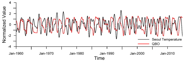
 and QBO (Temperature, Seoul)
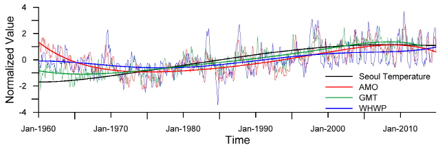
 , AMO, TNA, WHWP, and GMT (Temperature, Seoul)
적도 지역의 30 mb 고도에서의 위도 간 바람장으로 정의되는 QBO와의 상관관계는 10개월의 시간차를 두고 대체로 약 -0.3 정도에 해당하는 미세한 음의 상관관계를 나타내었다. QBO를 통해 적도 지역 성층권에서의 대기 움직임을 파악할 수 있는데, 이를 통해 적도 지역의 대규모 대기순환인 워커순환으로 표현되는 엘니뇨 남방진동의 현상을 관측할수 있다. 따라서 우리나라 기온과 상관관계를 보인다는 것을 통해서도 엘니뇨 현상이 우리나라의 기온 변동과 관련이 있음을 알 수 있다. 다음의 Fig. 5는 10개월 이전의 QBO와 서울지점 기온의  의 정규화된 시계열을 도시한 그림이다. 이를 통해 QBO와 기온간의 위상이 약하게 반대의 위상을 갖는 것을 확인할 수 있다.
추세를 의미하는 잔여요소에서는 강수와의 상관관계 분석 결과와 마찬가지로 대서양 해수면 온도와 관련된 AMO, Atlantic Tripole SST EOF, Caribbean Index, NTA, TSA, TNA 및 태평양 해수면 온도와 관련된 WHWP, Pacific Warmpool에서 시간차를 두지 않고 대체로 0.5 이상의 유의할 만한 상관계수를 나타내었다. 또한 전 지구적인 기온변화를 나타내는 GMT에서는 매우 높은 0.8 이상의 상관계수를 나타내었다. 이는 지구온난화로 인한 해수면, 기온상승의 추세가 우리나라 기온에도 영향을 미치고 있음을 의미한다. 다음의 Fig. 6은 서울지점기온자료의 진여요소와 AMO, WHWP, GMT의 시계열을 도시한 그림이다. Fig. 3과 마찬가지로 그림에서 표시된 굵은 선은 각 기상인자의 6차 다항 회귀식이다. 강수와 마찬가지로 기온자료 또한 증가하는 추세를 보이고 있으며 해수면 온도, 기온 관련 기상인자의 증가 추세와 일치하는 것을 확인 할 수 있다.
5. 결 론
강수 및 기온자료와 기상인자 간의 상관관계를 분석함에 있어서 강수 및 기온자료를 원 자료 그대로 분석을 수행 할 경우 실제로 명확한 상관관계를 찾아내기가 어렵다. 따라서 원 자료계열을 단순화 하거나 분해하여 여러 요소를 추출하는 방법을 통해 상관관계를 좀 더 명확히 할 필요가 있다. 본 연구에서는 경험적 모드분해법을 통해 기상청 14개 지점의 강수 및 기온자료를 주기별로 분해하여 내재모드함수를 추출하였다. 이를 해수면온도, 대기 순환, 강수 및 기온의 변화를 나타내는 다양한 기상인자와의 상관관계 분석을 통해 주기성과 경향성의 두 가지 측면에서 각 기상인자와 강수 및 기온간의 상관관계를 분석하여 다음과 같은 결론을 얻을 수 있었다.
1. 주기성과 관련하여 월총강수량의  의 경우 엘니뇨 관측에 사용되는 적도 지역 해수면 온도 관련 기상인자인 NINO 1+2, NINO 3.4, NINO 3과 각각 4개월, 3개월, 3개월의 시간차를 두고 유의할 만한 상관관계를 보였다. 이는 우리나라 강수의 장기적인 예측에 있어서 4개월 이전의 엘니뇨 현상의 관측을 통해 강수의 변화 양상을 추정할 수 있을 것으로 판단된다.
2. 기온의 경우 우리나라 월평균기온의  와 NINO 1+2, NINO 3.4, NINO 3간에 각각 4개월, 3개월, 3개월의 시간차를 두고 유의할 만한 상관관계를 나타냈다. 이는 엘니뇨 관측을 통해 기온의 변동을 예측할 수 있음을 보여주고 있다. 또한 기온과 적도 성층권 대기 순환을 의미하는 QBO와도 유의할 만한 상관관계를 보였다. 강한 엘니뇨가 발생할 경우 워커순환이 약해져 적도 지역의 대기 순환이 줄어들게 되어 엘니뇨 현상과 QBO 사이에는 반대의 위상을 갖는다는 점에서 QBO와 우리나라 기온이 음의 상관관계를 갖는다는 것은 우리나라 기상 변동이 엘니뇨 현상과 밀접한 관련이 있음을 보여준다.
3. 월총강수량 및 월평균기온 자료에서 모든 내재모드함수를 공제한 잔여요소와 대서양 및 태평양에서의 해수면온도, 전 세계적 기온변화를 의미하는 GMT와의 상관관계가 높게 나타나는 것을 통해 기후변화로 인해 나타나는 기온상승과 해수면 온도의 상승이 우리나라 기후변동과도 밀접한 관련이 있음을 확인 할 수 있다.
본 연구에서 사용된 경험적 모드분해법을 이용해 추출한 강수 및 기온자료와 기상인자의 상관관계 분석을 통해 주기성과 경향성 측면에서 좀 더 명확한 상관관계 분석이 가능한 것으로 판단되며, 향후 본 연구에서 분석한 상관관계를 바탕으로 기상인자를 통한 강수 및 기온의 예측 모형을 구축하는 연구가 진행되어야 할 것이다.
