

1. 서 론
2. Study Area and Dataset
2.1 Site description
2.2 Global Land Data Assimilation System (GLDAS)
2.3 MODIS GPP
2.4 Model description
2.5 In-situ downward shortwave radiation
2.6 In-situ gross primary production
3. Methodology
3.1 Structural equation modeling
3.2 Statistical methods
4. Results and discussion
4.1 Validation
4.2 Environmental variables influence to gross primary production in normal year
4.3 Environmental variables influence to gross primary production in drought
5. Conclusion
1. 서 론
The carbon storage in the ecosystem has experienced the carbon cycles in the exchange of plants, oceans, lands, atmosphere, and sub grounds. The carbon cycle is one of the major parts of the ecological cycles of the ecosystems (Grace, 2004), while the carbon fluxes from the atmosphere to the plants is called the Gross Primary Production (GPP), which is known as the main driver of the land carbon sink (Spielmann et al., 2019). The carbon flux including GPP is determined by the environmental variables such as shortwave downward radiation (RSD), vapor pressure deficit (VPD), air temperature (Tair) and evaporative fraction (EF) which are the main factors that have relationships with the plants physiological processes (Borges et al., 2017).
This interaction magnitudes between the GPP and environmental variables can be changed in different environmental state that can be high VPD or temperature environments. Pau et al. (2018) showed that the temperature has increased GPP until 35℃, but above 35℃, the temperature is negatively correlated to GPP. Goodrich et al. (2015) found that the high VPD had negative effects on the stomatal conductance for the plants to prevent the loss of transpiration and caused the decrement of GPP. Tabari and Aghajanloo (2013) separated dry condition periods by using aridity index in the Iran regions to analyze the trends of the aridity. Moreover, recent studies considered not only the correlations between GPP and environmental variables, but the dynamic interactions between the environmental variables in different environment conditions.
To date, ground estimation of GPP can be obtained from the eddy covariance flux towers that have high accuracy but limited spatial resolution to represent the regional scale of GPP especially in the heterogeneous terrain such as in South Korea. To represent the regional scale, the GPP estimations from remote sensing and land surface model simulation has been used (Stocker et al., 2019; Mu et al., 2007). Land surface model is a process-based model and simulates the fluxes of water and energy in the land-atmosphere interface. Community Land Model 4 (CLM 4) is one of land surface model and has been validated in previous studies for estimating the carbon fluxes (Mao et al., 2012; Hudiburg et al., 2013; Zhang et al., 2016). CLM 4 considers the exchange among the atmospheric fluxes, sub ground hydrologic conditions, and vegetation phenology reactions. For the satellite dataset-based estimation of GPP, Moderate Resolution Imaging Spectroradiometer (MODIS) GPP product (MOD17A2) has been widely used to estimate the carbon cycle in the regional or global scale (Yu et al., 2018).
However, the GPP estimation between the process-based model and satellite dataset-based model are different. CLM 4 uses the Biome-BGC model while MODIS algorithm uses Light Use Efficiency (LUE) model to estimate GPP. They also have different parameters, equations and input dataset, and it could lead to the differences of GPP responses toward the environmental variables (Mao et al., 2012). Previous studies found the differences of GPP sensitivities toward the change of environmental variables between satellite dataset based GPP estimation algorithms and process-based models by varying the input dataset (Dong et al., 2015; Williams et al., 2014). However, this method is time consuming work and more effort need to be done to consider the multivariable product such as GPP.
Structural Equation Modeling (SEM) method is for causal analysis and it can consider multivariable at low computational costs (Fan et al., 2016). The SEM use path analysis and can estimate the effects of each variable for specific conditions. This study used SEM with environmental variables such as Tair, VPD, RSD, and hydrologic factor of EF and dependent variable of GPP. The effects of each factor to the others were expressed as a path and the path coefficients are estimated by using the maximum likelihood estimation method. Another merit of SEM is to show the causal analysis with visualization. Each causal analysis of SEM can be expressed with figures and can be easily compared. Previous studies used SEM to conduct sensitivity analysis of GPP to environmental variables using flux tower dataset. Wang et al. (2019) used the SEM method to conduct causal analysis for each environmental factors to GPP and showed the changes of correlations between the environmental factors and the GPP in warm and cold years using flux tower observation dataset. Fu et al. (2020) used SEM with flux tower based observation dataset to show sensitivity analysis of GPP to environmental factors in drought season in Europe.
In Korea, GPP estimation studies were conducted with flux tower data in the Seolmacheon (hereafter SMC) site and Cheongmicheon (hereafter CMC) site (Shin et al., 2012; Jung et al., 2015; Huang et al., 2018). Jung et al. (2015) compared GPP products from MODIS to flux tower GPP estimation in the SMC and CMC sites, and found that GPP products from MODIS showed similar seasonal patterns with flux tower estimated GPP. Huang et al. (2018) used Breathing Earth System Simulator (BESS) process-based model to evaluate the GPP products of BESS and conducted sensitivity analysis of GPP to the environmental variables in the CMC site. However, the influences from environmental variables to GPP have not been studied yet. In this study, we used SEM techniques to analyze the impacts of different land covers and drought conditions to the influences of environmental variables to GPP products. The impacts were shown in SEM models with GPP measured from flux tower, MODIS, and CLM 4 and they were compared.
This study aims to compare the GPP products from multiple datasets and conduct the causal analysis for GPP with environmental variables by using the SEM analysis during the drought seasons at the SMC and CMC sites in South Korea. The specific purposes of this study are as follows: (1) to validate GPP products, EF and environmental drivers from in-situ dataset, (2) to analyze the effects of environmental drivers and EF to GPP and (3) to analyze the change of relationships between environmental drivers and EF to GPP in cropland and forest sites for drought period.
2. Study Area and Dataset
2.1 Site description
The flux towers located in SMC and CMC are measuring the hydrological indexes, carbon flux and energy fluxes. The details of measurements devices and the environments of the flux towers are shown in Table 1.
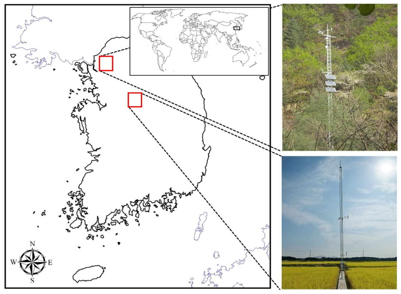
The field sites are SMC flux tower site and CMC flux tower site participated in Asiaflux in South Korea, located at the Gyeonggi-do Paju-si (37° 56' 20" N, 126° 57' 17" E) for SMC and at the Gyeonggi-do Yeuju-si (37° 9' 35" N, 127° 39' 10" E) for CMC (Fig. 1). SMC flux tower is located in the middle of the mountain and the vegetation type is mixed forest. CMC flux tower is located in the middle of the crop land area which is irrigated during the spring to the autumn. The mean annual temperature of SMC and CMC are 10.9℃ and 11.6℃. The mean annual precipitation of SMC and CMC are 1,458 mm yr-1, 1,370 mm yr-1 for each. The elevation of SMC is 293 m and CMC is 141 m. Both flux towers are operated by Korea Institute of Hydrological Survey. Flux tower data was measured by using the eddy covariance method. The data of CO2 flux, net shortwave radiation, Tair, VPD, sensible heat flux, latent heat flux, and friction velocity were extracted at a 30-min temporal resolution and were up-scaled to daily data.
When the flux tower data have missing values of more than 100 days, we excluded the whole year data for this study. Hence, we have excluded the flux tower data for SMC in 2013 and CMC flux tower data in 2016 for that particular reason. Overall, we used the flux tower data in 2012, 2014, 2015, and 2016 from SMC site and flux tower data in 2012, 2013, 2014, and 2015 from CMC site. Hong et al. (2016) showed that the Korean peninsula had severe agricultural drought in 2014 and 2015, hence, we used the data from 2014 and 2015 to study the changes of relationships between environmental drivers and GPP in drought years.
Table 1.
Measurement devices and observed dataset of flux towers of Seolmacheon and Cheongmicheon sites
2.2 Global Land Data Assimilation System (GLDAS)
The Global Land Data Assimilation System (GLDAS) provides land surface and near land surface atmosphere data by assimilating the observation-based data of land surface models namely Noah, CLM, Variable Infiltration Capacity (VIC), Mosaic, and Catchment land surface model (CLSM). GLDAS data includes the forcing data (e.g., precipitation, near-surface air temperature, specific humidity, wind speed, surface pressure, downward shortwave and longwave radiation), land surface state (e.g., soil moisture, surface runoff and subsurface runoff) and flux data (e.g., evaporation and sensible heat flux). From the source data, GLDAS products can be classified into GLDAS-1 version and GLDAS-2 version. GLDAS-1 provides reanalysis data from 1979 to present using ECMWF reanalysis data, NCEP-NCAR reanalysis data, NOAA/GDAS atmospheric analysis fields. GLDAS-2 provides data from 1948 to presents using Princeton meteorological forcing dataset (Sheffield et al., 2006). The GLDAS data can be accessed on online (http://disc.sci.gsfc.nasa.gov/hydrology/data-holdings). GLDAS-2.1 datasets has spatial resolution of 0.25° × 0.25° and 3 hourly temporal resolutions. In this study, we used environmental variables datasets from GLDAS-2.1 data products as forcing datasets for the CLM 4 from 2012 to 2016.
2.3 MODIS GPP
The Moderate Resolution Imaging Spectroradiometer (MODIS) instrument is aboard on Aqua and Terra satellites operated by National Aeronautics and Space Administration (NASA). This study used MOD17A2 GPP product (Collection 6), which has 8-day revisit time and temporal resolution of 500 m. MODIS GPP uses Light use efficiency (LUE) model to estimate daily GPP as shown in Eq. (1)
where max is maximum radiation use efficiency coefficient, f (Tmin) and f (VPD) are attenuation scalars controlled by daily minimum of air temperature (Tmin) and daily VPD for each, RSD is downward shortwave radiation (W m-2) and FPAR is fraction of absorbed photosynthetically active radiation. f (Tmin) and f (VPD) are to represent GPP attenuation in low temperature and high VPD situation. max is defined from Biome Parameter Look-Up Table (BPLUT) and the vegetation type is from MODIS land cover data (MOD12Q1). The data source of MODIS GPP is from MODIS data and reanalysis data. FPAR was obtained from MOD15 algorithm and Tmin, RSD and VPD data were obtained from reanalysis data.
2.4 Model description
The CLM 4 was developed as a sub-model of Community Earth System Model (CESM) by National Center for Atmospheric Research. It has ability to calculate the energy exchange mechanism between the land and atmosphere. CLM 4 requires the forcing datasets (i.e., pressure, temperature, solar incident shortwave radiation, solar incident longwave radiation, relative humidity, wind speed, and precipitation) to calculate the diverse hydrologic data. In this study, the forcing datasets were obtained from the GLDAS 2.1 datasets.
CLM 4 uses Biome-BGC model to simulate carbon and nitrogen dynamics on the terrestrial ecosystem. The carbon and nitrogen state variables distributed in the vegetation, litter and soil organic matter are simulated in spin-up timing. GPP is estimated in the process of growth and litter fall of plants in the CLM 4. Biome-BGC model has two water stress scalars to GPP which are VPD multiplier (MVPD) and soil-leaf water potential multiplier (MPSI). MVPD and MPSI are to represent attenuation of GPP in the situations of high VPD and low soil-leaf water potential (PSI). The total water stress scalar can be expressed as MVPD × MPSI. The MVPD estimation equation is shared in MODIS in the form of f (VPD).
To simulate CLM 4 process using flux towers, we selected BGC-CN mode, which simulates over 600 years to stabilize the environments states and obtain carbon flux datasets based on Biome-BGC model. In this study, we simulated the carbon fluxes and set the spin up period as 700 years to reduce the uncertainties in carbon fluxes and the CO2 concentration was fitted to 370 ppm which is the 10-year average in SMC flux tower. The more detail contents of CLM 4 are described in Oleson et al. (2010) and Lawrence et al. (2011).
2.5 In-situ downward shortwave radiation
Net shortwave radiation (W m-2) can be divided into downward shortwave radiation (W m-2) and upward shortwave radiation (W m-2) as Eq. (2)
where RSN is net shortwave radiation, RSD is downward shortwave radiation and RSU is upward shortwave radiation. The RUD can be expressed with albedo and RSD as Eq. (3)
where is land surface reflectance (albedo) and this study used MODIS albedo estimated from MCD43A1. MCD43A1 has spatial resolution of 500 m and temporal resolution of daily.
2.6 In-situ gross primary production
GPP is the sum of net ecosystem exchange (NEE) and ecosystem respiration (Re) as described by Taylor et al. (2000) as Eq. (4)
where, the NEE has negative values for the absorbed CO2 mass on the designed volume, but Re has plus values for estimating the used CO2 mass by the plants.
In general, the eddy covariance method based flux tower used the mass conservation equation for estimating NEE as shown in Eq. (5).
In Eq. (5), FCT is turbulent flux of carbon flux and FCS is storage flux of carbon flux. We assumed that the atmospheric turbulence was sufficient in the SMC and CMC sites, and advection fluxes were assumed negligible (Aubinet et al., 2012). FCT can be estimated from flux tower measurements and FCS was calculated based on an assumption that CO2 concentration estimated from flux tower can represent the CO2 concentration values in whole layers below the eddy covariance system (Flanagan et al., 2002). FCS can be estimated as following Eq. (6)
where h is height of top of the flux tower which is 19.2 m for SMC and 10.0 m for CMC sites and c is the change of CO2 concentration (mol m-3). In the flux tower estimation, CO2 concentration was measured in mg m-3 and it was converted to mol m-3 by using ideal gas law equation.
To determine the atmospheric turbulence condition, we used friction velocity threshold. The friction velocity was measured from the flux towers and we determined the atmospheric turbulence condition to be sufficient when the friction velocity was larger than 0.2 m s-1. The gaps of the NEE data were filled with extrapolation methods which are descripted as Falge et al. (2001).
The NEE can be partitioned to GPP and Re, and the Re was estimated from the nighttime NEE estimation. During the nighttime, GPP can be assumed to be zero (Lasslop et al., 2010), and the absolute values of NEE and Re are equal. We extrapolated Re to daytime periods with the equation suggested by Lloyd and Taylor (1994) as shown in Eq. (7)
where Re,ref is base respiration at the reference temperature (Tref) which is set to 15℃, and E0 is the temperature sensitivity, Tair is air temperature, and T0 is -46.02℃. In this study, the NEE partitioning process was conducted by using the ‘ReddyProc’ package in R (Wutzler et al., 2018).
3. Methodology
3.1 Structural equation modeling
To determine the differences of the correlations between the hydrological variables (i.e., VPD, EF, RSD and Tair), the SEM metrics were employed in this study. The SEM is statistical model that is used for causal analysis for multivariate mechanism. The SEM can be a solution for explaining the complex mechanisms between the GPP and other environmental factors, and the SEM considers the covariance between the factors and shows the direct effects and indirect effects of variables (Wang et al., 2019).
This study, we used model fit indexes such as χ2 test of the model fit (P) and the adjusted goodness of fit index (AGFI) and root mean square error of approximation (RMSEA) for evaluation of SEM model. To evaluate SEM to be “good fitting”, P should be over 0.05, AGFI should be less than 0.9, and RMSEA should be less than 0.08 (Grace, 2006).
The strengths of connections between the components are represented as path coefficients. To estimate path coefficients, the covariance matrices are computed based on the observed data and structural model each, and the path coefficients are estimated by minimizing the differences of covariance from the observed data and covariance implied by the structural model. Path coefficient is standardized values, and the magnitude of the path coefficients shows that the effective connectivity. When the coefficient is close to the 1 or -1, the relationship is strong in positive or negative. The merit of the SEM is to calculate the direct effects and indirect effects. More detailed information of SEM can be found in the previous studies by Wang et al. (2019).
In this study, SEM to the GPP was conducted with in-situ dataset and regional scale datasets (MODIS, GLDAS, and CLM 4 dataset) at SMC site and the CMC site. The set explanatory variables to be RSD, EF, Tair and VPD and the dependent variable to be GPP. We constructed SEM models which were for in-situ GPP (hereafter FLUX GPP), MODIS GPP, and CLM GPP. In the SEM for FLUX GPP, environmental drivers and EF were from in-situ dataset. The first SEM used flux tower observation dataset of EF, Tair, VPD and in-situ estimation dataset of RSD and GPP. We assumed that hydrological parameters from GLDAS dataset can represent the environmental drivers and EF data in the regional scale. In the SEM for MODIS GPP and CLM GPP, environmental drivers and EF were from GLDAS dataset. The SEM model with in situ GPP and environmental variables can represent the plant phonological processes in SMC and CMC sites. SEM models with MODIS GPP and CLM GPP be compared to the SEM model with FLUX GPP and it could make to find the errors of MODIS GPP and CLM GPP. To fit the spatiotemporal resolutions between the environmental variables and the GPP, we unified spatial resolution of MODIS GPP to 25 km. The SEM shows the path coefficients for the significant paths between the variables. The path coefficient is standardized and it has -1 to1 values. The AGFI, P-value and RMSEA fit indexes for the SEM are used in this study to test the model fit.
3.2 Statistical methods
To validate the GLDAS and CLM 4 data with flux tower observation dataset, Pearson correlation coefficient (R), root mean square error (RMSE), and bias were used. These can be calculated by using the Eqs. (8) ~ (10) as follows
where M is predicted value, O is measurement values and n is the total number of compared data. Each of are mean of predicted values and measurement values.
4. Results and discussion
4.1 Validation
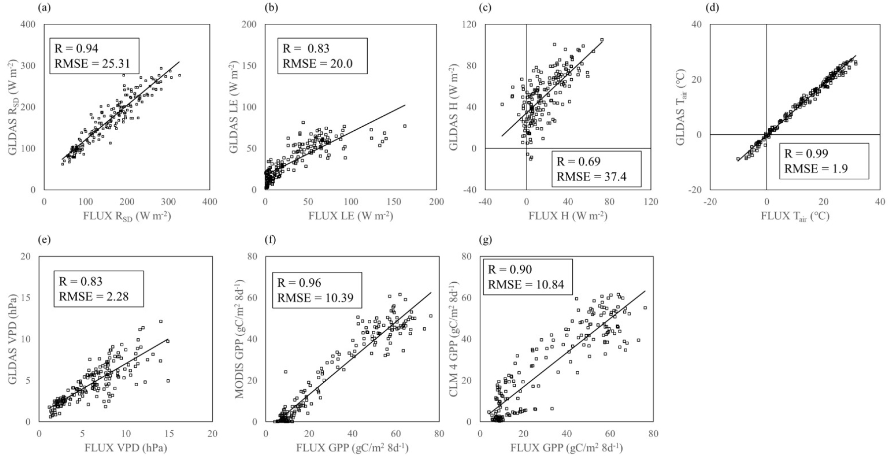
We validated the RSD, H, LE, VPD, Tair, and GPP of MODIS and CLM 4 dataset with in-situ dataset at SMC site and CMC site as shown in Figs. 2 and 3. The environmental variables and GPP data has different spatiotemporal resolutions, but the different spatiotemporal resolutions could make uncertainties for making covariance matrices in the SEM models. To make the same spatiotemporal resolution for the regional scale dataset, MODIS GPP values in the pixels of 25 km × 25 km was averaged in the SMC site and CMC site and the averaged MODIS GPP data were used in the SEM models. The temporal resolutions of the GLDAS data and CLM GPP are daily and MODIS GPP data is 8 days. In the SEM models, GLDAS data was averaged to 8 days and CLM GPP data was sum to 8 days. GLDAS dataset and GPP dataset from MODIS and CLM 4 (hereafter CLM GPP) were validated with the in-situ observation from the flux tower with statistic values of RMSE and R.
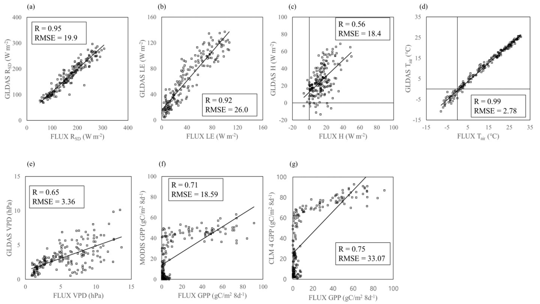
Table 2 is showing R, RMSE and bias for each environmental drivers, MODIS GPP and CLM GPP. The validation results of RSD and Tair from GLDAS showed good agreement with flux tower observation in both sites with the R values of RSD and Tair that were same or larger than 0.94. The index of RMSE of RSD and Tair also showed good results with values of 25.31 W m-2, 32.3 W m-2 for RSD in SMC and CMC sites, and 1.9℃, 2.78℃ for Tair in SMC and CMC sites each. GLDAS also showed reasonable agreement with the in-situ dataset for LE, H, and VPD at SMC and CMC sites with relatively high values of R, RMSE, and bias, as shown in Table 2. However, VPD was underestimated in CMC site with low value of R. This can be caused from the spatial resolution of GLDAS, because the heterogeneous terrain in the CLM site may cause some interruption for the GLDAS result.
MODIS GPP and CLM GPP were consistent with the flux tower GPP in SMC site. The results demonstrated good values of R and RMSE as shown in Table. 2. In CMC site, MODIS GPP and CLM GPP showed overestimation compared to the flux tower GPP, especially for the low values. This may be caused from the spatial resolution of vegetation types inherent to CLM 4 and MODIS GPP algorithms. The environments in the 25 km × 25 km grid cell centered of SMC is almost consists of mixed forest land cover and similar to the environments of the SMC flux tower. On the other hand, the 25 km × 25 km grid cell centered of CMC site is mixed with mixed forest and cropland. However, the flux tower of CMC site is located in the cropland and it could lead the overestimation of GPP in CLM 4 and MODIS caused by high values of fraction of photosynthetically active radiation absorbed by the canopy (Turner et al., 2006). The transplant time of rice in the CMC site is from mid-May to mid-late September (Huang et al., 2018). On the other hand, the growing season of forest and grassland starts on April and end in October. This overestimation of GPP products from CLM and MODIS can be shown in Fig. 3.
Table 2.
Statistical methods (R, RMSE, bias) for validating GLDAS dataset of downward shortwave radiation (RSD), LE, H, VPD, Tair, MODIS GPP, and CLM GPP at SMC site and CMC site
4.2 Environmental variables influence to gross primary production in normal year
Droughts occurred in Korean peninsula in 2014 and 2015. In this study, we divided the periods to be normal and drought years. Data from normal year in the SEM models were from 2012, 2016 for the SMC site and 2012, 2013 for CMC site. Fig. 4 showed SEM structures for GPP derived from in situ GPP (hereafter FLUX GPP), MODIS GPP, and CLM GPP with RSD, Tair, EF, and VPD. SEM for FLUX GPP, the environmental variables were obtained from in-situ dataset. While SEM for MODIS GPP and CLM GPP, the environmental drivers and EF were obtained from GLDAS.
In the in-situ data based SEM models (Figs. 4(a) and 4(d)) showed Tair was a main driver for FLUX GPP with path coefficient () of 0.76 in SMC and 0.84 in CMC. RSD had significant effect towards FLUX GPP, but its magnitude of path coefficient was less than 0.2 in the SMC site and it was negative in the CMC site. In the CMC site, the rice was usually transplanted in mid-May and harvested in mid-late September (Huang et al., 2018). The negative direct path coefficients of RSD to FLUX GPP come from the spring and late autumn seasons which showed low GPP values and high RSD values. VPD had direct effect to FLUX GPP at SMC site, but at CMC site, it only had indirect effect through EF. EF also had direct effects to FLUX GPP, however, it was not statistically significant in both sites (P > 0.05). RSD and Tair in the CMC sites affected less to EF rather than in the SMC site, because the irrigation can reduce the effects of Tair and RSD to the available soil moisture. Im et al. (2014) showed that irrigation can affect surface energy partitioning and this changed energy partitioning can reduce effects from Tair and RSD to EF. Moreover, the irrigation relieved VPD effects to FLUX GPP. In the SMC site, VPD had direct effect to FLUX GPP, but in the CMC site, the VPD had indirect effect only. The irrigated lands has low VPD values rather than non-irrigated lands (Ambika and Mishra, 2020). The low values of VPD led to lower effects of VPD to FLUX GPP in the CMC site.
The GLDAS environmental variables based SEM models with MODIS GPP (Figs. 4(b) and 4(e)) and CLM GPP (Figs. 4(c) and 4(f)) showed that GLDAS RSD has high value of path coefficient ( = 0.41-0.73) towards MODIS GPP and CLM GPP. In the CMC site, in-situ estimated RSD had negative effect to FLUX GPP, but GLDAS RSD had positive effects to the MODIS GPP and CLM GPP, because the 25 km × 25 km grid cell of CMC site not only contain cropland, but also forest, grassland, and wetlands. This caused the mismatch of growing seasons for the plants. MODIS GPP has overestimation trends in mid-growing season and outside the growing seasons (Turner et al., 2006) Forest and grassland have broader growing seasons (April to October) rather than the actual rice growing seasons (from May to September). It made MODIS GPP and CLM GPP to be well consistent to the interannual trend of RSD. GLDAS Tair had insignificant path coefficient towards MODIS GPP and CLM GPP, because in both algorithms, the Tair is not directly used to estimate GPP, but the minimum of Tair is treated as restriction of GPP. GLDAS EF had significant path coefficient towards MODIS GPP and CLM GPP and the path coefficients of GLDAS EF was overestimated ( = 0.31-0.37). This means that the MODIS GPP and CLM GPP used energy balances to estimate GPP in their algorithms. The paths of GLDAS VPD to MODIS GPP and CLM GPP were different to the paths of in situ estimated VPD to the FLUX GPP in both sites. GLDAS VPD had negative direct path coefficient to MODIS GPP and CLM GPP in CMC, but in SMC site, GLDAS VPD did not have direct path coefficient towards MODIS GPP and only had indirect effect through EF. This means that the water stress represented by VPD was not accurate in the MODIS GPP and CLM GPP. It can be related to the underestimation of GLDAS VPD. GLDAS VPD was underestimated in both sites and Malek-Madani et al. (2020) showed that underestimation of VPD can induce the inaccurate water stress condition at field sites. MODIS GPP and CLM GPP commonly used VPD scalar to express water stress, and VPD scalar is determined by minimum of daily VPD (VPD_min) and maximum of daily VPD (VPD_max) by the BPLUT. In the mixed forest and cropland, VPD_min is 6.5 hPa and VPD_max is 24 hPa for mixed forest and 43 hPa for cropland. However, GLDAS VPD is underestimated as shown in Fig. 6. This can be a reason of errors of estimating MODIS GPP and CLM GPP.
The differences between the SEM models with MODIS GPP and CLM GPP come from the structures of GPP estimation algorithm (Mao et al., 2012). LUE based GPP estimation model used RSD and VPD data. but they did not include the EF and Tair. Biome-BGC models use combination of the MVPD and MPSI. However, the path coefficients of SEM models with MODIS GPP and CLM GPP were similar. They are less affected from the variability of Tair and if they have underestimated VPD data as the forcing dataset, it could lead errors for estimating GPP.
In Table 3, we can see the total effects (TF) of environmental variables to all GPP products. RSD and Tair were found as the main drivers of GPP (TF = 0.33-0.76 for RSD, TF = 0.28-0.88 for Tair) in all types of GPP. The direct effect of RSD was largely estimated in the MODIS GPP and CLM GPP, because they use RSD as an input data and are dependent on RSD data. Interestingly, the in situ observed RSD had negative direct effect to FLUX GPP at CMC site, but for total effects, RSD had subsequent positive values. This was caused from the strong direct effect values of Tair to FLUX GPP. Direct effect of Tair was stronger than GLDAS Tair to GPP and the indirect effects of RSD through the Tair to GPP was estimated relatively stronger.
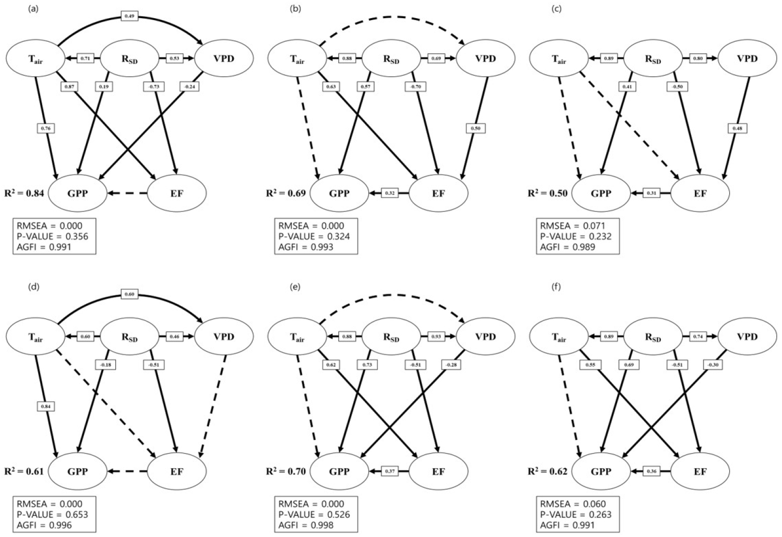
Fig. 4.
Structural equation model (SEM) for 8-day sum gross primary production (GPP) with environmental drivers and evaporative fraction (EF) derived from 8-day average dataset of flux tower, MODIS, GLDAS, and CLM 4 in normal years (2012, 2013 and 2016) at SMC and CMC sites. For SMC site, the GPP was derived from (a) flux tower, (b) MODIS, and (c) CLM 4. For CMC site, the GPP was derived from (d) flux tower, (e) MODIS, and (f) CLM 4. The types of lines indicate significant paths (solid lines, P < 0.05) and insignificant paths (dotted lines, P > 0.05) in the model and the standardized path coefficients are located in the significant paths. Model fit indexes such as Root Mean Square Error Approximation (RMSEA), chi-square p-value and Adjusted goodness of fit index (AGFI) of each SEM models were shown below the SEM
Table 3.
Effects of environmental factors to GPP in normal seasons (2012, 2016 for SMC and 2012, 2013 for CMC). Significant effects (P < 0.05) are denoted by bold.
4.3 Environmental variables influence to gross primary production in drought
Drought in Korean peninsula was occurred in 2014 and 2015. During this period, the annual precipitation amounts were half of the average annual precipitation. Fig. 5 showed the SEM results, similar to Fig. 4, but during the drought season in 2014 and 2015. The SEM structures for FLUX GPP were not changed, but the path coefficients values were changed. RSD had strong effects towards FLUX GPP in both sites. Compared to normal years, path coefficients of RSD for FLUX GPP in drought period was changed from 0.19 to 0.40 in SMC and from -0.18 to -0.33 in CMC. In 2014 and 2015, the number of clear days was higher compared to the normal season, and it reinforced the RSD effects. During the drought season, RSD had stronger path coefficient not only towards FLUX GPP, but also towards the other environmental variables such as VPD and Tair. Path coefficients of Tair to FLUX GPP was similar to normal season, but the path coefficient to EF was changed to significant path coefficient at CMC site. Path coefficients of EF to FLUX GPP was insignificant which is same to normal years. Direct effects of VPD to FLUX GPP was not changed a lot. This results are consistent to the results of previous study. Fu et al. (2020) reported that VPD effects to GPP in the drought season was similar to the VPD effects to GPP in normal season.
The SEM results from the MODIS GPP SEM and CLM GPP SEM also showed that the path coefficient from Tair to GPP was changed from insignificant to significant. GLDAS RSD was changed from a dominant driver of MODIS GPP and CLM GPP products to one of the main drivers of environmental variables to MODIS GPP and CLM GPP products. The magnitude of the direct effects from environmental variables to MODIS GPP and CLM GPP were reduced compared to normal years, but path coefficient of GLDAS Tair to MODIS GPP and CLM GPP was increased in both sites. Path coefficient of RSD to MODIS GPP and CLM GPP decreased compared to normal years, because the drought lowered radiation use efficiency (Fu et al., 2020). Path coefficient of GLDAS EF to MODIS GPP and CLM GPP also reduced, but it is still overestimated compared to direct effect of in situ estimated EF to FLUX GPP. Path coefficients of GLDAS Tair to MODIS GPP and CLM GPP increased compared to normal years, because of the reduced amounts and frequency of precipitation. Yu et al. (2017) showed that reduced precipitation amounts, and frequency sustains high air temperature and it enhance the correlations between the Tair and GPP. GLDAS VPD direct path to MODIS GPP and CLM GPP was moved to EF in the drought season.
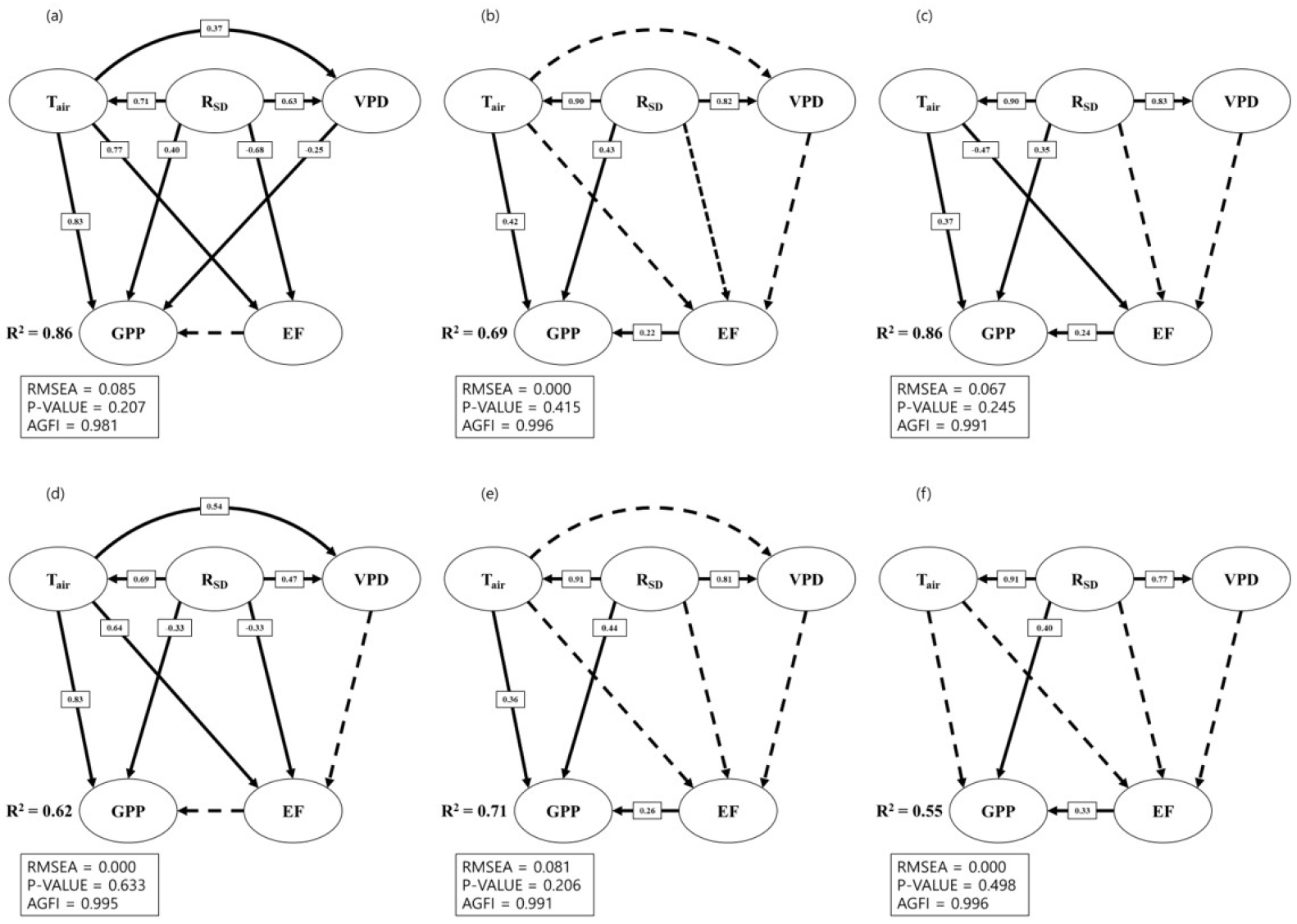
Fig. 5.
Structural equation model (SEM) for 8-day sum gross primary production (GPP) with environmental drivers and evaporative fraction (EF) derived from 8-day average dataset of flux tower, MODIS, GLDAS and CLM 4 in drought years (2014 and 2015) at SMC and CMC sites. For SMC site, the GPP was derived from (a) flux tower, (b) MODIS, and (c) CLM 4. For CMC site, the GPP was derived from (d) flux tower, (e) MODIS, and (f) CLM 4. The types of lines indicate significant paths (solid lines, P < 0.05) and insignificant paths (dotted lines, P > 0.05) in the model and the standardized path coefficients are located in the significant paths. Model fit indexes such as Root Mean Square Error Approximation (RMSEA), chi-square p-value and Adjusted goodness of fit index (AGFI) of each SEM models were shown below the SEM.
Fig. 6 shows that box plots of interannual VPD estimated from flux tower and GLDAS in normal years and drought years. In drought season, the frequency and amount of precipitation were reduced, and it caused high air temperature and it also increased GLDAS VPD. In the drought season, GLDAS VPD annual variations were ranging from 1 hPa to 12 hPa in SMC and 1 hPa to 10 hPa in CMC, while in normal season the GLDAS VPD annual variations were ranging from 1 hPa to 10 hPa and 1 hPa to 6 hPa in CMC. However, it is still low values to restrict GPP as following the VPD_min and VPD_max descripted in BPLUT. Therefore, the GLDAS VPD does not have negative effects to MODIS GPP and CLM GPP in both sites.
Table 4 shows the total effects of the environmental variables towards GPP during the drought season in 2014 and 2015 at SMC and CMC. Path coefficients of RSD to GPP in drought season remains unchanged, but the direct and indirect effect towards GPP were changed. The reduced direct effects of RSD towards GPP were recovered by the indirect effects through EF and Tair. However, in SMC site, path coefficients of in-situ environmental variables towards GPP were not significantly changed, and the direct effect of RSD in drought season was increased, but the indirect effect of RSD was decreased, so the total effects of RSD to FLUX GPP was not relatively changed. Path coefficient of EF to FLUX GPP was increased compared to normal years ( = 0.03 to 0.04 in SMC and = 0.08 to 0.18 in CMC). In the drought season, water stress increased and sensitivity of GPP to soil moisture increased (Fu et al., 2020). In drought season, the VPD effects to GPP was not significantly estimated except for SMC site for the in-situ data driven SEM results.
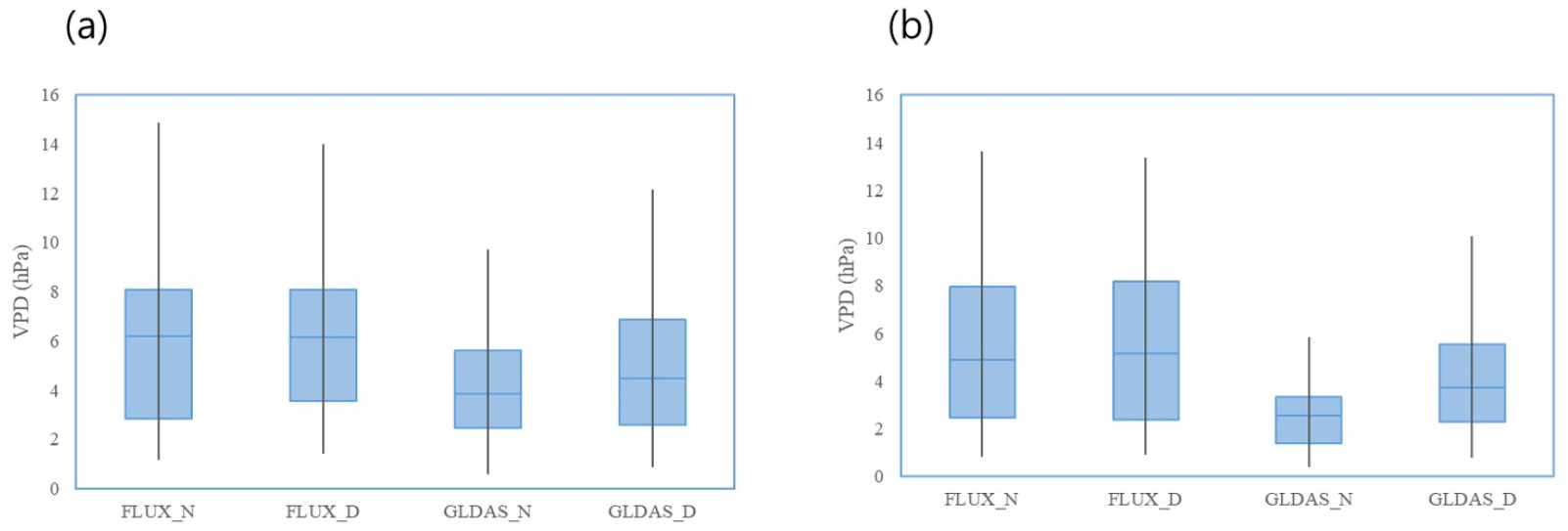
Table 4.
Effects of environmental factors to GPP in drought season in 2014 and 2015 for SMC and CMC. Significant effects (P < 0.05) are denoted by bold
5. Conclusion
We compared the SEM model derived from in-situ dataset and regional scale dataset such as CLM 4, MODIS, and GLDAS at different spatiotemporal resolutions. MODIS GPP is based on LUE model and CLM GPP is based on Biome-BGC model. LUE based model assumed that estimated fraction of absorbed photosynthetically active radiation and VPD are relatively accurate, and they do not consider GPP response to low soil moisture. This might cause errors of MODIS GPP especially during the drought period. To avoid that problem, we included EF data which represents available soil moisture in the land. We assumed that GLDAS has similar results of input data of MODIS GPP and further evaluated by using SEM analysis to show causal analysis of the environmental variables towards MODIS GPP and CLM GPP products.
This study showed that transplant time of rice should be calibrated for MODIS GPP and CLM GPP before estimate GPP products. The 25 km × 25 km grid size of MODIS GPP and CLM GPP not only contained cropland, but also forests, grassland, and wetland. This brought differences of growing season periods. The mismatch of sprout time of rice in CMC site brought negative direct effects of RSD to FLUX GPP. In the CMC site, the effects from Tair and RSD to EF can be reduced from irrigation. Irrigation directly supplies water to the soil and it can improve available water contents. Moreover, the irrigation made differences of effects of VPD to FLUX GPP. Irrigation can sustain values of VPD low and it weakens VPD effects to FLUX GPP in the CMC site. GPP estimated from MODIS and CLM were well consistent to the trend of RSD and it overestimated RSD effects to GPP. Otherwise, Tair was not used directly to estimate GPP in the algorithms of MODIS and CLM, but minimum of daily Tair was used. This reduced the effects of Tair to GPP products. MODIS and CLM used energy balance equations to estimate environmental drivers, the effects of GLDAS EF to MODIS GPP and CLM GPP were overestimated. GLDAS VPD was underestimated, and it reduced the effects of VPD to GPP. GPP estimation algorithms including LUE-based GPP model and Biome-BGC based GPP model showed similar responses to the change of environmental variables.
During the drought season, the frequency and amounts of precipitation reduced and it enlarge the magnitude of effects of RSD to GPP. This drought environments sustain high values of GLDAS Tair and it led high values of GLDAS VPD. However, the daily GLDAS VPD was not extreme to restrict GPP and the GLDAS VPD effects to GPP was not significant. In the drought season, plants were more sensitive to soil water contents and our results showed that effects of EF to GPP were enlarged. Drought also reduced radiation use efficiency and the direct effects of GLDAS RSD to GPP products were reduced in drought season. Further studies should consider the irrigation effects and accuracy of VPD data for estimating GPP products from MODIS and CLM.
