

1. Introduction
2. Study Area
2.1 Habitat and Hydrologic Data
2.2 Physical Habitat Simulation
3. Results
3.1 Scenario 1 and Scenario 2 using the Building Block Approach
3.2 Changes in CSI and WUA
3.3 Change of Economic Outcomes
4. Conclusions
1. Introduction
Physical habitat simulation is a numerical approach that quantifies the relationship between particular discharge and physical habitat for an aquatic species (Bovee, 1982; Booker and Dunbar, 2004). Thus, it is capable of investigating the impact of a change in flow on habitat availability and suitability for target species. Physical habitat simulation is mainly composed of hydraulic simulation and habitat simulation. Hydraulic simulation computes not only physical habitat variables such as flow depth, velocity, and substrate but also bed elevation change for a given discharge. Habitat simulation predicts habitat quality and quantity for aquatic species on the basis of the species’ preference of each physical habitat variable.
Physical habitat simulations have been successfully used to various relevant problems. The environmental flows in rivers was estimated using physical habitat simulation (Freeman et al., 2001; Acreman and Dunbar, 2004; Nikghalb et al., 2016). Using physical habitat simulation, the results of designing a river restoration (Frissell et al., 1986; Im et al., 2011), evaluate river health (Maddock, 1999), and to assess the impact of river works (Yi et al., 2010; Chang et al., 2013). Later, physical habitat simulation was applied to impact of flow regime change by dam construction (Valentin et al., 1996; Yi et al., 2010; Choi et al., 2017; Kang et al., 2017; Choi and Choi, 2018). Similarly, the change of dam operation was investigated with respect to ecological requirements of downstream from the dam (Poff et al., 1997; Postel and Richter, 2003; Zhang et al., 2017).
Most physical habitat simulations are highly dependent on the given discharge, especially, regulated river by upstream dam. Flows regulated by upstream dams affect the downstream habitat in hydropeaking (Valentin et al., 1996) and thermopeaking (Ward and Stanford, 1979). Dams can significantly change the flow regime such as timing, frequency, and duration of low flows and high flows (Poff et al., 1997; Bunn and Arthington, 2002; Richter et al., 2003; Postel and Richter, 2003; Richter et al., 2006). Many previous studies investigated that hydropeaking flows (Valentin et al., 1996; Korman and Campana, 2009; Booker and Dunbar, 2004; Garcia et al., 2011; Chen et al., 2015; Choi et al., 2017) and thermopeaking flows (Lessard and Hayes, 2003; Li et al., 2011; Zolezzi et al., 2011; Boavida et al., 2015; Kang et al., 2017; Choi and Choi, 2018) reduces habitat suitability for target species in the downstream reach. However, most previous physical habitat simulations have not taken designing dam re-operations into account when assessing the effect that hydropeaking flows have on the downstream habitat (Poff et al., 1997; Richter et al., 2003; Postel and Richter, 2003). In addition, the one of the primary goal of the hydropeaking is to maximize the utilization of economic benefits. Changes in the amount of water released from the dam and timing may affect the economic benefit. In recent years, the optimal goals of dam operation are shifting from single objective to multiple objectives. That is, it is great necessity to change the operation of the dam considering both ecological and economic benefits. This is motivated the present study.
The goal of this study was to investigate the impact of designing dam operation through the natural flow regime on environmental and economic benefits. For this, a 3.35 km long reach in the Dal Stream, Korea, was selected. This study reach is a gravel-bed stream located downstream from the Goesan Dam. For the physical habitat simulation, Zacco platypus, Zacco temminckii, Coreoleuciscus splendidus, and Opsariichthys bidens were selected as the target species in the study reach. Physical habitat simulations were carried out using the River2D model and the HSI model for hydraulic and habitat simulations, respectively. For the HSI (Habitat Suitability Index) model, HSCs (Habitat Suitability Curves) were constructed using the method of Gosse (1982), and the scenarios of the modification of dam re-operations were proposed using the BBA. First, the impact of modifying dam operation through the natural flow regime in physical habitat simulations was examined quantitatively. Then, the hydroelectric power benefits change with the designing dam re-operation was presented, and predicts the environmental and economic benefits were compared.
2. Study Area
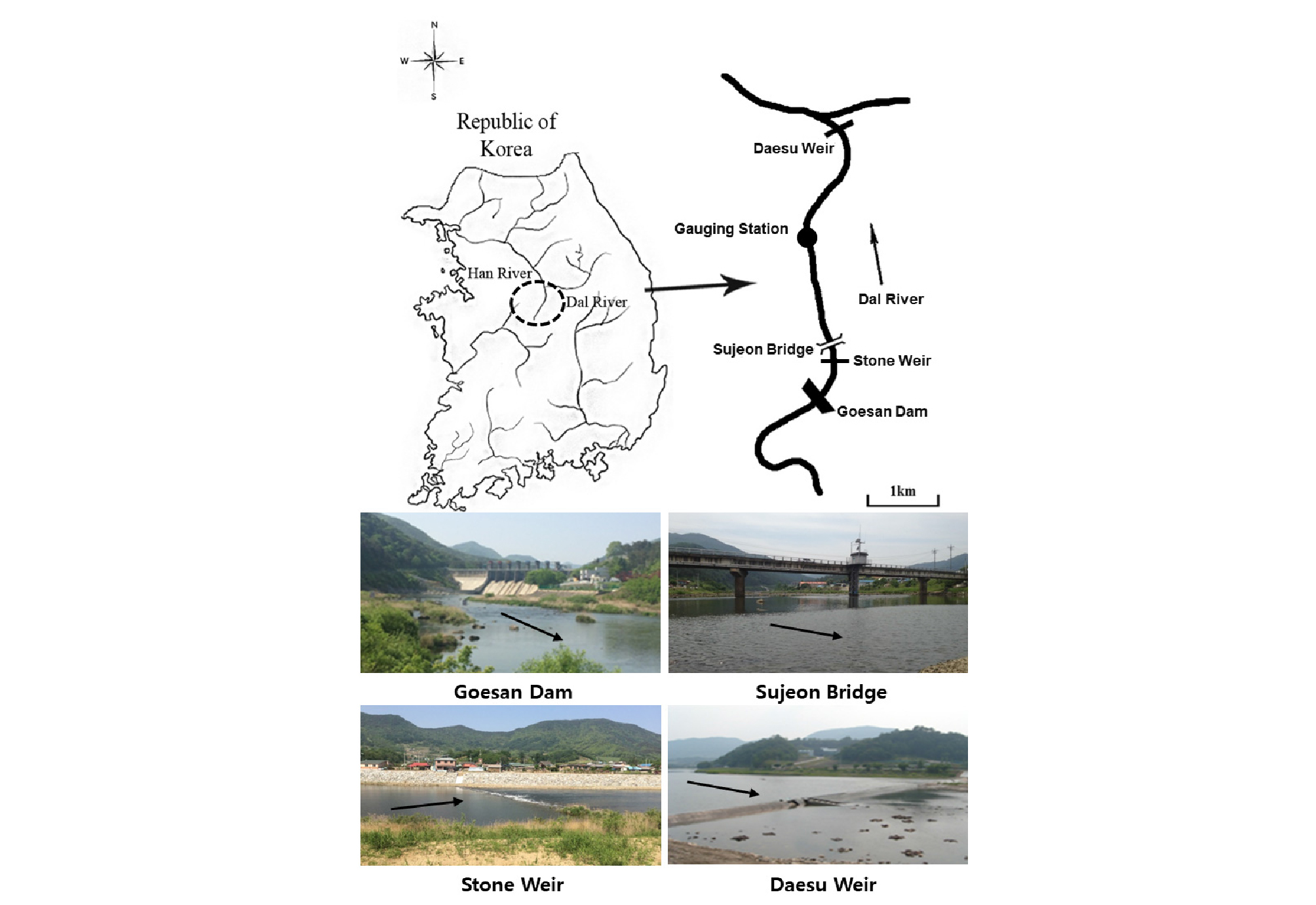
This study area in the Dal Stream, Korea is located downstream from the Goesan Dam as shown in Fig. 1. The dam was constructed in 1957 and has a total storage capacity of 1.53 × 10⁶ m3. The study reach is 3.35 km long, extending from the Goesan Dam to the Daesu Weir. The average bed slope of the reach is about 1/650. The Goesan Dam, located 1.05 km upstream from the Sujeon Bridge, regulates the flow in the study reach. Also, small artificial stone weir, located 0.6 km downstream from the Goesan Dam, which maintain upstream flow depth as 1.0 m at low flow regime. The dam discharges water only during hydropower generation. Consequently, the Daesu Weir maintains flow constant, even when the dam is not discharging water. For the study reach, the discharges for drought flow (Q355), low flow (Q275), normal flow (Q185), averaged-wet flow (Q95) are 1.82, 4.02, 7.23, and 17.13 m3/s, respectively (Ministry of Construction and Transportation, 1995). Here, Qn denotes the average discharge which is exceeded on n days of the year.
2.1 Habitat and Hydrologic Data
For the period of 2007-2010, hydrologic and fish monitoring data were collected for the study reach through Government R&D projects (Ministry of Science and Technology, 2007; Ministry of Land, Transport and Maritime Affairs, 2011). To measure the water surface elevation, various devices such as float-type, sonar, and radar water gauge were installed at the Sujeon Bridge. Velocity was measured using Price current meter. Fish monitoring was carried out using cast nets and kick nets, revealing that dominant species in the study area Zacco platypus, followed by Coreoleuciscus splendidus, and Zacco temminckii (see Fig. 2). They account for 27%, 15%, and 15%, respectively, of the population (Ministry of Land, Transport and Maritime Affairs, 2011). The total number of 1492 datasets were used for the physical habitat simulation in the present study. In this study, not only the dominant species but also an indigenous species were selected as the target species.

Through field investigations, Kim et al. (2007) indicated that the bed materials in the study reach ranges from sand to cobble. The median size of bed sediment is 137 mm, revealing that the study reach is a gravel-bed stream. A riffle is located in the straight reach just upstream from the bend and pools are present before and after this riffle. Bed sediment particles are also affected by the morphology of the stream, resulting in the occurrence of coarse and fine particles at the riffle and pools, respectively (Kim et al., 2007). Kim et al. (2007) reported that the median size of the bed sediment particles in the riffle is 166 mm, and the bed sediment particles in the pool ranges between 60 and 120 mm.
2.2 Physical Habitat Simulation
2.2.1 Hydraulic and Bed Elevation Simulation
In the present study, the River2D model was used for the hydraulic and bed elevation simulation. The model was developed by Steffler and Blackburn (2002). The River2D model is capable of computing transient turbulent flows in an open-channel. Also, The River2D model offers both wet and dry solutions, by changing the surface flow equations to groundwater flow equations in dry area The River2D model solves two-dimensional depth-averaged shallow water equations using the finite element method. The continuity and longitudinal (x) and lateral (y) components of momentum equations are given by, respectively,
| $$\frac{\partial H}{\partial t}+\frac{\partial q_x}{\partial x}+\frac{\partial q_y}{\partial y}=0$$ | (1) |
where t is the time, x and y are the streamwise and transverse directions, respectively, H is the flow depth, U and V are the depth-averaged velocities in the x- and y-directions, respectively, qx and qy are respective discharges per unit width (qx = HU, qy = HV), g is the gravitational acceleration, is the water density, S0i and Sfi are the river bed slope and friction slope in the i-direction, and ij is the horizontal turbulent stress tensor. The x- and y-components of the friction slope in Eqs. (2) and (3) are expressed by, respectively,
| $$S_{fx}=\frac{n^2\;U\sqrt{U^2+V^2}}{H^{4/3}}$$ | (4a) |
| $$S_{fy}=\frac{n^2\;V\sqrt{U^2+V^2}}{H^{4/3}}$$ | (4b) |
where n is the Manning’s roughness coefficient. The two-dimensional bedload sediment continuity equation for the bed elevation change is given by
| $$(1-\lambda)\frac{\partial z_b}{\partial t}+\frac{\partial q_{sx}}{\partial x}+\frac{\partial q_{sy}}{\partial y}=0$$ | (5) |
where qsx and qsy are the components of volumetric rate of bedload transport per unit length in the x- and y-directions, respectively. λ is the porosity of the bed material, t is time and zb is the bed elevation. In the present study, the formula by the Müller et al. (1948) is used to estimate the transport rate qsx and qsy for a sediment mixture in Eq. (5).
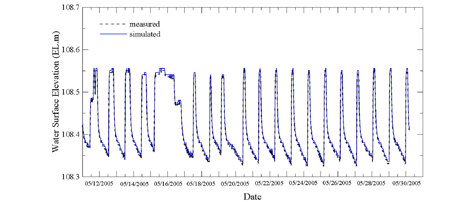
Validation of the 2D unsteady flow model was performed, and result is given in Fig. 3. Fig. 3 shows the change of the water surface elevation due to the hydropeaking flows for May 12-May 31, 2005. The water surface elevation simulated using the River2D model is compared with the measured data (Kim et al., 2011). The measuring station is located 1.05 km downstream from the Sujeon Bridge (see Fig. 1), and the water surface elevations were measured with an air purge level gauge (Kim et al., 2011). In the present computation, values of Manning’s n ranging between 0.039-0.052, which were obtained through calibration by Kim et al. (2007). The dam discharged hydropeaking flows 19 times during this period with a peak discharge of about 15 m3/s. It can be seen that the predicted water surface elevation is in good agreement with the measured data. This indicates that the River2D model is capable of simulating short-term fluctuating flows due to hydropeakings in the downstream reach from the dam.
2.2.2 Habitat Simulation
In the present study, the HSI model was used for habitat simulations. HSI model were developed to characterize habitat quality for selected target species. HSI models describe the relationship between habitat variables and the suitability. The HSI is a numerical value ranging from zero to unity, representing unsuitable and optimal habitat, respectively. The HSI model is assumed to have a positive linear relationship with the potential carrying capacity of the habitat (U.S. Fish and Wildlife Service, 1981). In this study, to construct the HSCs, the method proposed by Gosse (1982) was used. This method gives values of suitability index 1.0, 0.5, 0.1, and 0.05 to the range of variable that encompasses 50%, 75%, 90%, and 95% of the observations, respectively.
The habitat suitability was evaluated via habitat simulation based on the monitoring data. In general, the results of the habitat simulation are given by CSI (Composite Suitability Index) and WUA. The WUA is calculated by multiplying the CSI by the area of the cell.
| $$WUA={\textstyle\sum_{i=1}^n}\;A_i\times CSI_i=f(Q)$$ | (6) |
where CSIi is the value of the CSI of cell i, Ai is the area of i-th computation cell, and Q is the discharge. The WUA provides information regarding the amount of discharge required to maintain the optimal conditions for physical habitats. For calculating the CSI, the multiplicative aggregation method was used. In this study, two habitat variables such as flow depth and velocity were used. This is because most of the target species does not have a substrate preference (Yeom et al., 2007; Hur and Seo, 2011; Hur et al., 2011; Choi and Choi, 2015).
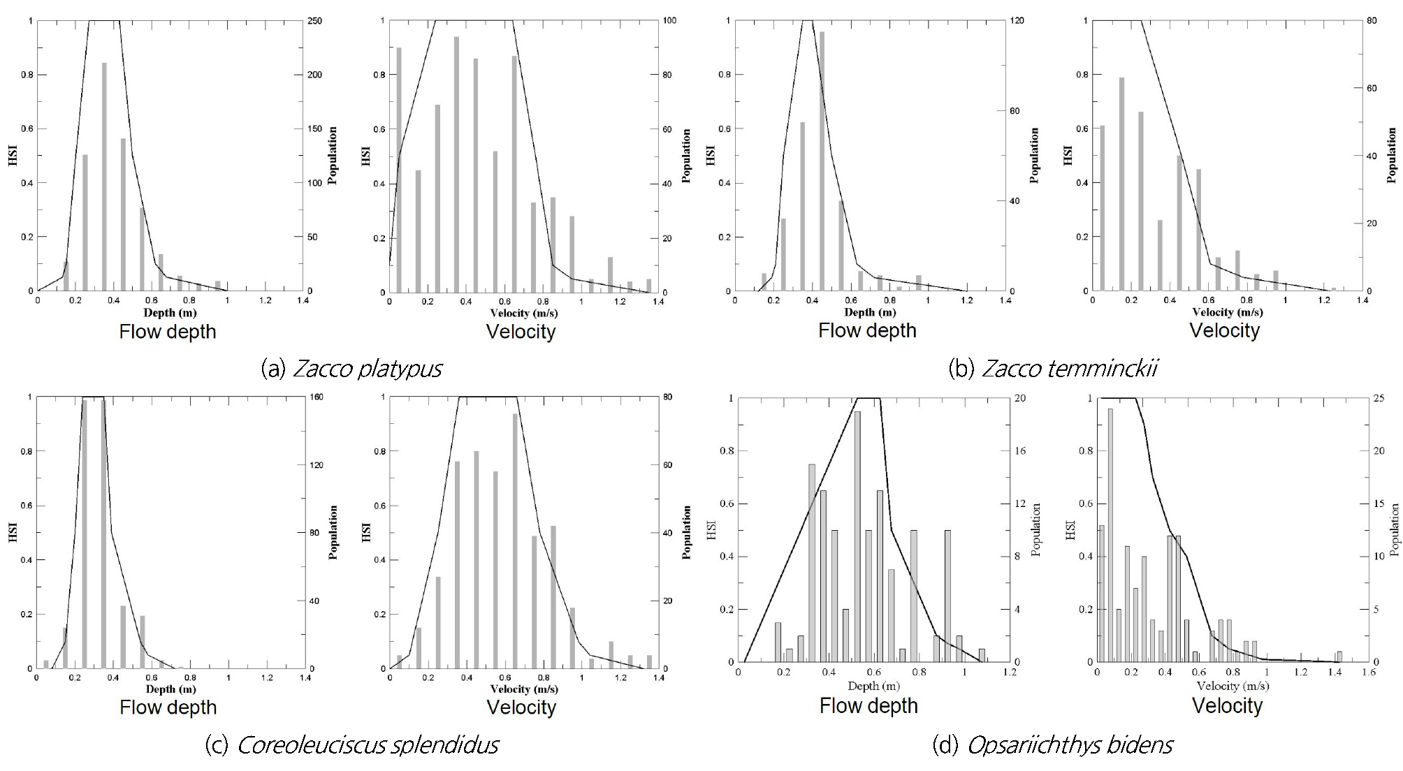
The individual HSC for the target species in the Dal Stream was constructed using the method of Gosse (1982) are given in Figs. 4(a)~4(d). In the figure, the population of the fish is also given for each range of physical habitat variable. With these HSCs, the CSIs were calculated using the multiplicative aggregation method later. The plots that Zacco platypus prefers a flow depth range of 0.3-0.5 m and a velocity of 0.2-0.55 m/s. For Zacco temminckii, the respective ranges are 0.35-0.4 m and 0-0.25 m/s, respectively. For Coreoleuciscus splendidus and Opsariichthys bidens, the respective preferred ranges are 0.25-0.35 m and 0.5-0.65 m for flow depth and 0.35-0.45 m/s and 0.05-0.25 m/s for velocity. It is interesting to note that the ranges of the velocity preferred by each target species are clearly different, but the ranges of the flow depth are not.
3. Results
3.1 Scenario 1 and Scenario 2 using the Building Block Approach
The Building Block Approach (BBA) was introduced for modifying dam operations using the hydrologic and ecological data (Tharme and King, 1998). The approach is one of the holistic methods for estimating environmental flows (King and Louw, 1998; Postel and Richter, 2003). The procedures of modifying dam operations using the BBA can be divided into the following three steps: (1) defined as the minimum in-stream flows using the averaged the hydrologic data over the each month, (2) building the flushing flood for channel maintenance and habitat improvement, and (3) Increasing the discharge in dry season for spawn habitat and migration. Also, Postel and Richter (2003) introduced modified dam operation scenarios based on the natural flow regime. They proposed four methods, namely static minimum flow allocation, percent of flow allocation, seasonally adjusted minimum flow allocation, and seasonally adjusted minimum flow allocation with seasonal flushing flow.
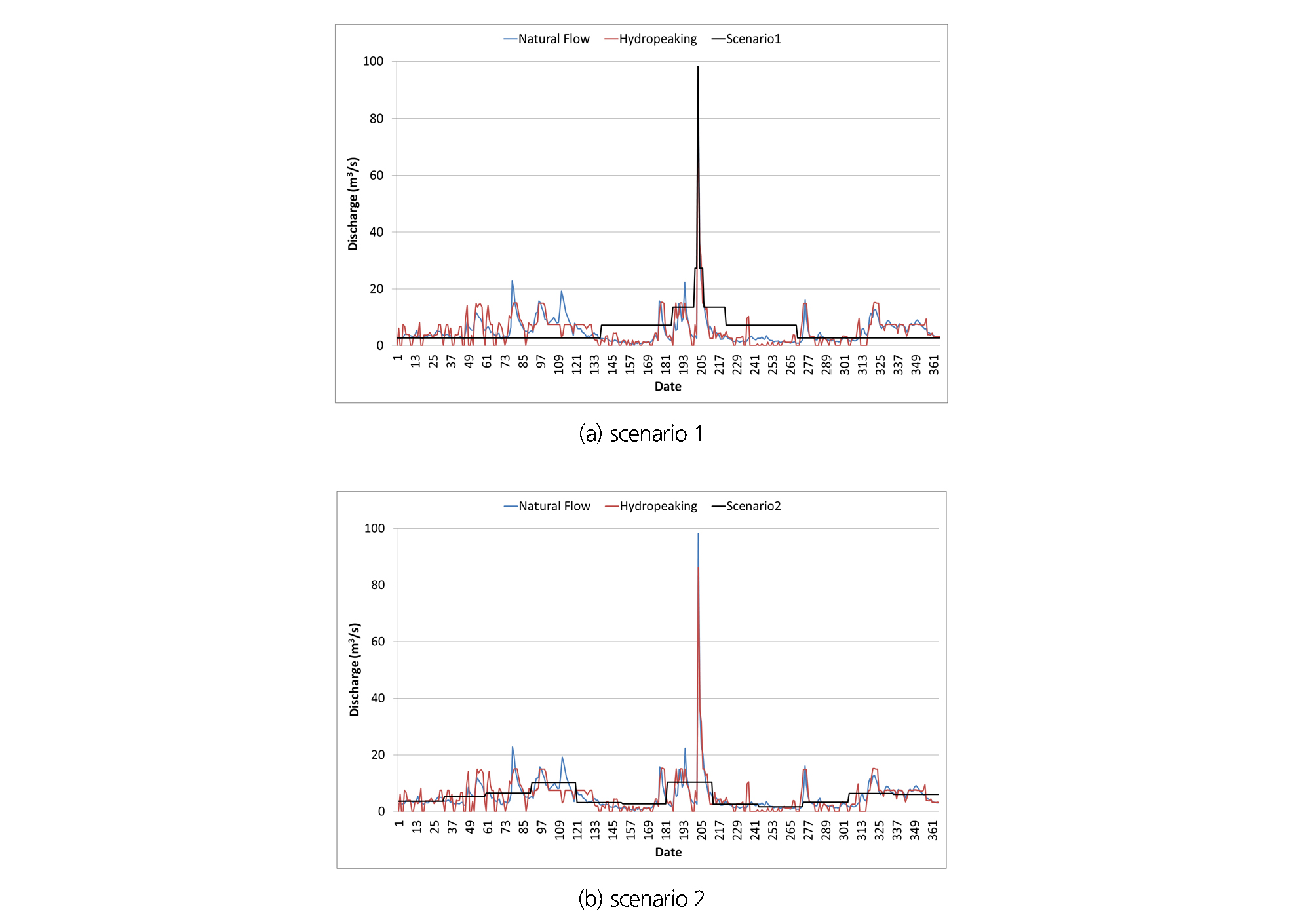
In the present study, among the several methods, two methods were used, namely magnitude-duration concept and seasonally adjusted minimum flow allocation concept. The figures (Figs. 5(a) and 5(b)) are the scenario 1 and 2 for the physical habitat simulation using the BBA. For comparisons, the natural flow regime and hydropeaking flows are provided. The natural flow regime and hydropeaking flows refer to the inflow from the upstream reach to the dam and the water released from the upstream dam, respectively. Fig. 5(a) shows the scenario 1 using analysis of the magnitude and duration for the hydrologic data. In the figure, the scenario 1 is composed of the low flows events, high flow events, and flood events. The peak discharge of the scenario 1 is 98 m3/s in June. Also, Fig. 5(b) shows the scenario 2 using the seasonally adjusted minimum flow allocation, i.e., averaged the hydrologic data over the each month. In general, the scenario 2 is composed of the low flows events and high flow events. The total volume of the scenario 1 and scenario 2 is about 1.41 × 10⁶ m3 and 1.48 × 10⁶ m3, respectively, which is very close to the volume of 1.53 × 10⁶ m3 released from the dam.
3.2 Changes in CSI and WUA
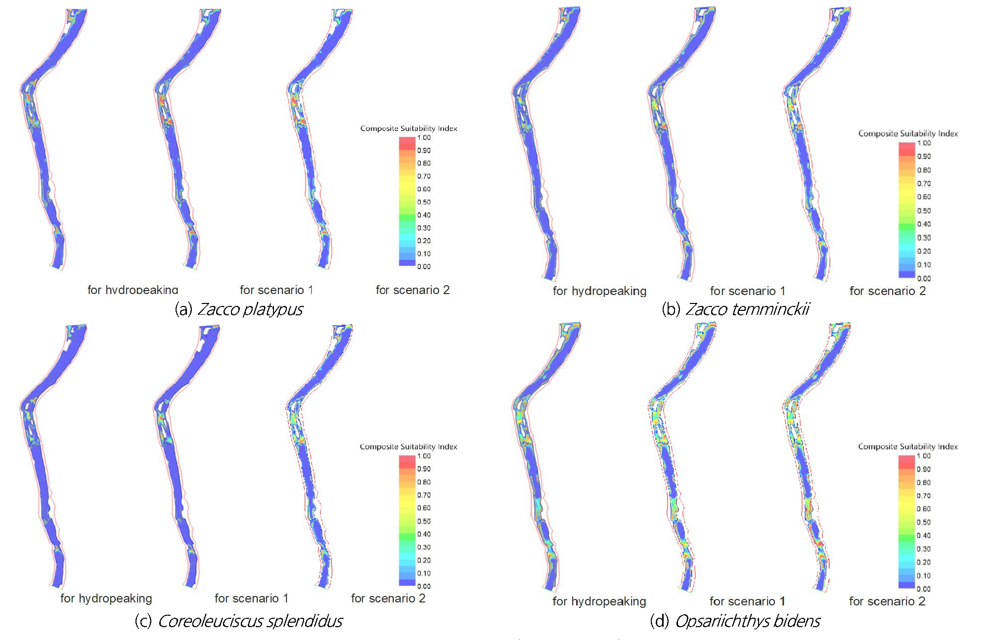
Figs. 6(a)~6(d) shows the CSI distributions predicted by the HSI model for hydropeaking flows, scenario 1, and scenario 2, respectively. The CSI ranges from zero to unity, indicating the worst and most optimal habitat conditions, respectively. The CSI distributions predicted from the habitat simulations with HSCs by the method of Gosse (1982) in Fig. 4. In each case, the computed CSI distributions are averaged over the year. A general trend observed in the figure is that the distributions of the CSI for the three cases are similar. Fig. 6 shows that the scenario 1 and scenario 2 significantly increased the CSI when in comparison to the CSI distribution for the hydropeaking conditions. Specifically, CSI is high in the vicinity of the bend and in reaches close to both ends. This is because the physical habitat suitability is extremely low for the base flow during the hydropower generation recession period and this recession period is prevalent during the entire period, as seen in Fig. 5. This result is consistent with the previous findings of studies performed by Garcia et al. (2011), Winterhalt (2015), and Choi and Choi (2018).
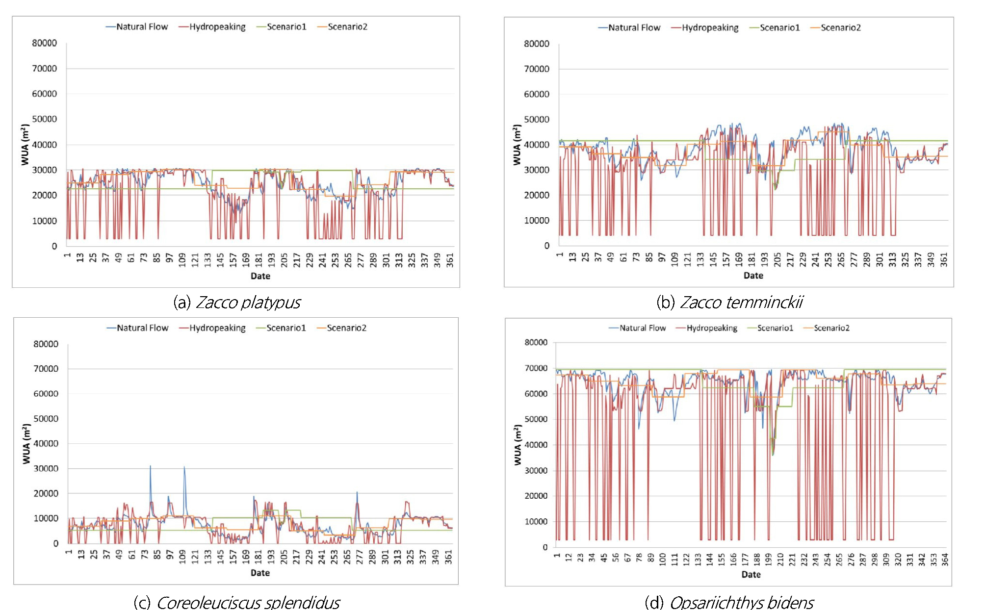
The change in the WUA with time is presented in Figs. 7(a)~7(d). In the figure, for comparisons, the WUA with the natural flow regime and hydropeaking flows are also given. It can be seen in Figure that, in general, the WUA with hydropeaking effect is significantly smaller than the WUA for the scenario 1 and scenario 2. Quantitatively, the scenario 1 increase the WUA by 14.69%, 16.40%, 9.34%, and 30.62% for the Zacco platypus, Zacco temminckii, Coreoleuciscus splendidus, and Opsariichthys bidens, respectively. Also, the scenario 2 increases the WUA by 18.32%, 18.71%, 11.85%, and 28.93% for the Zacco platypus, Zacco temminckii, Coreoleuciscus splendidus, and Opsariichthys bidens, respectively. This indicates that the scenario 1 and scenario 2 beneficially affects the habitat suitability of the target fishes. The results demonstrate clear evidence that the modifying the dam operation through restoration to natural flow patterns are more advantageous not only dominant species but also an indigenous species.
3.3 Change of Economic Outcomes
The upstream dams have long been performed as providing hydropower generation and water supply. However, most dams were designed without taking into account the aquatic habitats of downstream from the upstream dams. Flow regulated by the upstream dam results in hydropeaking flows due to hydropower generation, which is significantly different from the natural flow regime. Changes in the flow regime due to designing of dam-re operation may affect the aquatic habitat in the downstream from the dam (Cowx et al., 1998; Korman and Campana, 2009; Li et al., 2011; Tuhtan et al., 2012; Boavida et al., 2015; Choi et al., 2017; Kang et al., 2017; Choi and Choi, 2018). In addition, designing of dam re-operation provides an opportunity to minimize economic outcomes. That is, results from a restoration of dam re-operation policy is not only aquatic ecosystems but also economically desirable.
Fig. 8 shows the hydroelectric power cost benefits with discharge in the study area. This data in Fig. 8 were observed from 2008 to 2017. It can be seen in Fig. 8 that the hydroelectric power benefits changes with the discharge. That is, it shows that the hydroelectric power cost benefits have various values even at the same discharge. This is due to that the economic factors to generate hydroelectric power each time and season are different. A general feature observed in the figure is that the hydroelectric power benefits tend to increase as the discharge increases. The correlation between hydroelectric power benefits and discharge was provided using a linear relationship, which was used in this study.
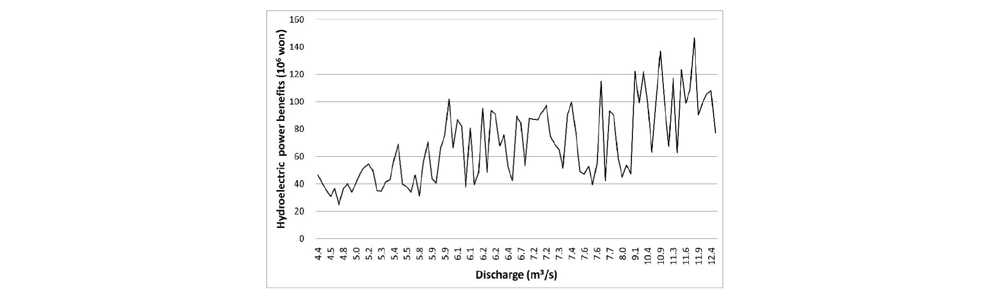
Fig. 9 shows the normalized hydroelectric power benefits for hydropeaking, scenario 1, and scenario 2, respectively. In each case, hydroelectric power benefits obtained from Figs. 5 and 8 are compared. That is, the quantity of total discharge is computed first by Fig. 5. Then, hydroelectric power benefits are computed by using linear relationship in the Fig. 8. Fig. 9 shows that the both scenarios decreased hydroelectric power benefits when in comparison to the benefits for the hydropeaking flows. Quantitatively, the designing of dam re-operation scenarios decrease the hydroelectric power benefits by 30.34% and 24.54%, respectively. This is due to that most of the total discharges of the each dam re-operation scenario are smaller than the hydropeaking except for some periods. However, except for the flood season, increasing the discharges from the dam at the level of the hydropeaking flows could bring nearly the same level for the hydroelectric power benefits, but the habitat for the target species increased by only about 5%. The results demonstrate clear evidence that modification of dam re-operation approach of storing and releasing water in time and volume is essential for balancing environmental and economic conditions.

Conclusions
This study conducted physical habitat simulations to investigate the impacts of modifying dam operation through the natural flow regime on downstream habitat. The study area is a 3.35 km long reach located downstream from the Goesan Dam in the Dal Stream, Korea. Zacco platypus, Zacco temminckii, Coreoleuciscus splendidus, and Opsariichthys bidens were selected as the target species in the study reach. The River2D model was used to predict the flow, and the HSI model was used for the habitat simulation. Two habitat variables, flow depth and velocity, were used in the physical habitat simulations. Validation of the River2D model was carried out with the hydropeaking flows, and the results indicate that the numerical model is capable of simulating short-term fluctuating flows. For the four target species, the method of Gosse (1982) was used to construct HSCs.
Scenario 1 and scenario 2 were proposed by using the hydrological regime and averaged the hydrologic data over the each month, respectively. The CSI for the target species in the study area was predicted for hydropeaking flows, scenario 1, and scenario 2 by the HSI model. The results indicate that the scenario 1 and scenario 2 significantly increased the CSIs when in comparison to the CSI distribution for the hydropeaking flows. Also, the changes in the WUA with time for the target species were investigated. Quantitatively, the scenario 1 and scenario 2 increases the WUA by about 17.76% and 19.45% for the target species, respectively. This indicates that the natural flow pattern have a significant effect on habitat suitability.
Finally, the hydroelectric power benefits change with each scenario was investigated. In general, it was shown that the economic benefits were increased gradually as dam released water increased. The change of normalized hydroelectric power benefits were provided for hydropeaking and both scenarios. It is noteworthy that the impact of hydropeaking mitigation scenarios on the environmental and economic benefits changes depending on the storing and releasing water in time and volume. On average, 27% of the economic outcomes decreased due to dam re-operation change in the study area. This indicated that the designing dam re-operation effect should be considered in the assessment of environmental and economic benefits due to restoration of natural flow regime.
