Comparative study of laminar and turbulent models for three-dimensional simulation of dam-break flow interacting with multiarray block obstacles

Asrini Chrysanti; Yangheon Song; Sangyoung Son

doi:10.3741/JKWRA.2023.56.S-1.1059

Preview

Research Article

Journal of Korea Water Resources Association. 31 December 2023. 1059-1069
https://doi.org/10.3741/JKWRA.2023.56.S-1.1059

Comparative study of laminar and turbulent models for three-dimensional simulation of dam-break flow interacting with multiarray block obstacles

다층 블록 장애물과 상호작용하는 3차원 댐붕괴흐름 모의를 위한 층류 및 난류 모델 비교 연구

Asrini Chrysanti^a^b

Yangheon Song^c

Sangyoung Son^d^*

크리산티 아스리니^a^b

송 양헌^c

손 상영^d^*

^aLecturer, Faculty of Civil and Environmental Engineering, Institut Teknologi Bandung, West Java, Indonesia

^bPh.D Candidate, School of Civil, Environmental and Architectural Engineering, Korea University, Seoul, Korea

^cResearcher, Coastal Hydrodynamics Lab., Korea University, Seoul, Korea

^dProfessor, School of Civil, Environmental and Architectural Engineering, Korea University, Seoul, Korea

^a반둥공과대학교 수자원공학연구그룹 강사

^b고려대학교 건축사회환경공학부 박사과정

^c고려대학교 해안유체역학연구실 연구원

^d고려대학교 건축사회환경공학부 교수

^{*Corresponding Author}

ABSTRACT

Dam-break flow occurs when an elevated dam suddenly collapses, resulting in the catastrophic release of rapid and uncontrolled impounded water. This study compares laminar and turbulent closure models for simulating three-dimensional dam-break flows using OpenFOAM. The Reynolds-Averaged Navier-Stokes (RANS) model, specifically the k-ε model, is employed to capture turbulent dissipation. Two scenarios are evaluated based on a laboratory experiment and a modified multi-layered block obstacle scenario. Both models effectively represent dam-break flows, with the turbulent closure model reducing oscillations. However, excessive dissipation in turbulent models can underestimate water surface profiles. Improving numerical schemes and grid resolution enhances flow recreation, particularly near structures and during turbulence. Model stability is more significantly influenced by numerical schemes and grid refinement than the use of turbulence closure. The k-ε model’s reliance on time-averaging processes poses challenges in representing dam-break profiles with pronounced discontinuities and unsteadiness. While simulating turbulence models requires extensive computational efforts, the performance improvement compared to laminar models is marginal. To achieve better representation, more advanced turbulence models like Large Eddy Simulation (LES) and Direct Numerical Simulation (DNS) are recommended, necessitating small spatial and time scales. This research provides insights into the applicability of different modeling approaches for simulating dam-break flows, emphasizing the importance of accurate representation near structures and during turbulence.

Keywords

Dam-break flow

Lamina model

RANS model

k-ε model

Flow-structure interaction

댐붕괴흐름은 댐이 갑자기 붕괴하여 제어가 어려운 상태의 고속흐름이 방출되는 현상이다. 이 연구에서는 3차원의 댐붕괴흐름을 모의하기 위해 OpenFOAM을 사용하여 층류 및 난류 모델을 적용하고 그 결과를 비교하였다. 난류 모의를 위해 레이놀즈 평균 나비에-스토크스 (Reynolds-Averaged Navier-Stokes) 모델, 구체적으로 k-ε 모델을 사용하였다. 수리모형실험과 함께 수정된 다층 블록 장애물 시나리오를 대상으로 두 가지 모델을 평가하였다. 두 모델 모두 댐붕괴흐름을 효과적으로 재현하였으며, 난류 모델은 흐름의 변동성을 감소시키는 역할을 보여줬다. 그러나 난류 모델에서의 과도한 에너지소산은 수위를 과소 평가하게 하는 것으로 나타났다. 수치기법 및 격자 해상도를 개선하여 적용한 결과 흐름재현성이 향상되었는데 이는 특히 구조물 근처의 난류흐름에서 두드러졌다. 모델 안정성의 경우 난류모델의 사용여부보다는 수치기법 및 격자 해상도의 개선에 더 크게 영향을 받았다. k-ε 모델에 내재된 시간평균처리의 특성은 불연속성과 불안정성이 두드러진 댐붕괴흐름을 재현하는 데 한계가 있음을 나타냈다. RANS 모델을 포함한 난류모의는 방대한 계산자원이 필요하지만, 층류 모델과 비교하여 성능 향상이 제한적이었다. 댐붕괴흐름을 정확히 재현하기 위해 LES (Large Eddy Simulation) 및 DNS (Direct Numerical Simulation)과 같은 고급 난류 모델의 사용이 권장되며, 이를 위해서는 미세한 공간 및 시간 스케일의 구성이 필수적이다. 이 연구를 통해 댐붕괴흐름을 모의할 때 기본적으로 사용할 수 있는 주요 접근법과 적용가능성을 측정하였으며, 구조물 근처에서 난류흐름에 대한 정확한 표현의 중요성을 강조할 수 있었다.

키워드

댐붕괴흐름

OpenFOAM

층류모델

난류모델

k-ε 모델

흐름-구조물 상호작용

MAIN

1. Introduction
2. Methodology
2.1 General description of OpenFOAM
2.2 Governing equations
2.3 Turbulence Modeling
2.4 Numerical schemes and solving procedures
2.5 Model setup
3. Numerical Results
3.1 Scenario 1 - Isolated obstacle
3.2 Scenario 2 - Multi-layered obstacles
4. Discussion
4.1 Numerical schemes and solving procedure
4.2 Model set-up
4.3 Laminar and RANS model
5. Conclusion

1. Introduction

Dam-break flow is an instantaneous flow resulting from the sudden collapse of high dams. The phenomenon leads to the catastrophic flow which releases a sudden, rapid and uncontrolled impounded water. Such rapid flows are observed to have a similarity to the tsunami flow which can induce a high impact force and a bore on a horizontal bed (Chanson, 2006). In addition, those floods could generate a high impact risk of flood hazard to the downstream area. When the developed area existed in the downstream area of the dam, the high-risk of the flood hazard increased. Therefore, the study of the dam-break flow characteristics can play an important role in giving a recommendation for mitigation framework purposes.

The studies of dam-break can be estimated by numerical simulation or experimental studies. Experimental studies on the dam-break flow characteristics over the obstacle and various geometry have been studied (Soares-Frazão and Zech, 2002, 2007; Soares-Frazão, 2007; Evangelista, 2015; Robb and Vasquez, 2015). Most of previous works on numerical models utilized the shallow water equation (SWE) to represent the dam-break flow (Evangelista, 2015; Robb and Vasquez, 2015). Although the result from these models shows reasonable performance, the computational fluid dynamics (CFD) in 3D simulation has become a prominent tool for solving the complex fluid flow problems. In the idealized dam-break case, the high-gradient existence may generate the high velocity acceleration and violate the shallow water assumptions (Biscarini et al., 2010). The influence of an obstacle to the dam-break flow also generates a high curvature of a free surface and non-hydrostatic vertical acceleration in the adjacent area to the obstacle (Aureli et al., 2015).

The dam-break flow can be laminar and turbulent. Previous studies have been interested in comparing the SWE with several turbulence closure models to compare the model accuracy (Biscarini et al., 2010; Kocaman et al., 2020; Hien and Van Chien, 2021; Liu et al., 2016; Rodríguez-Ocampo et al., 2020). The Reynolds-Averaged Navier Stokes (RANS) have been considered in many applications. The k-ε model has proven to simulate the shear flows quite accurately and thus widely used in the free flow region (Higuera et al., 2013). Although the SWE shows its applicability to simulate the dam-break flows, the dam-break flows are instinctively fully 3D processes with significant air entrainment (Kocaman et al., 2020). The strong unsteady, high turbulence mixed flow and shock waves might be developed in the dam-break flow, especially under the complex topography. Considering the development of computation efforts in recent days, the simulation of the 3D turbulence model is now accepted and continues as a subject of interest of many researchers. One example may be found from studies that have applied the turbulent closure model to simulate the dam-break flows in the swash zone and their relationship with groundwater flow (Kim et al., 2017; Delisle et al., 2023). However, despite the favorable agreement with experimental data observed through the incorporation of turbulent closure, the significance of turbulence modeling in dam-break flows also still arguable, especially in real and practical cases. Therefore, in this study the dam-break flow will be simulated in 3D model using OpenFOAM by comparing the laminar and turbulent closure models. Two scenarios will be compared following the laboratory experiment conducted by Soares-Frazão and Zech (2007) and the modified scenario of multi-layered obstacle, and the results will be discussed.

2. Methodology

2.1 General description of OpenFOAM

OpenFOAM has been widely used as one of the prominent tools to solve complex CFD problems. OpenFOAM offers the advantage of being a free and open-source software. The software allows the non-black-box method, which allows users to tailor the solvers based on their specific needs by changing the source code. The OpenFOAM employed the finite volume method (FVM) based on the discretization with the volume of fluid (VOF) method (Rusche, 2002). The VOF method allows the multiphase simulation in which the interface is not explicitly computed but utilizes the property of the phase fraction field over the fluid volume fraction. The VOF method should have the advantage to simulating the dam-break case with a sharp interface between two phases of water and air (Hien and Van Chien, 2021). InterFoam solver was utilized in this study to solve the three-dimensional Reynolds Averaged Navier-Stokes (RANS) for two incompressible phases using the finite volume method (FVM) and the volume of fluid (VOF). InterFoam supports several laminar and turbulence models such as k-ε, k-ω SST, and LES.

2.2 Governing equations

The 3-D numerical model carried out in this study is governed by the complete equations of Reynolds-Averaged Navier Stokes (RANS) for Newtonian, viscous and incompressible fluid as follows:

(1)

\nabla ∙ U = 0

(2)

\frac{\partial ρ U}{\partial t} + \nabla ∙ (ρ UU) - \nabla ∙ ((μ + μ_{t}) S) = - \nabla p + g X \nabla ρ + σ κ \nabla α

(3)

S = \frac{1}{2} (\nabla u + \nabla u^{T})

where U = velocity vector field (m/s); 𝜌 = density (kg/m³), 𝜇 = dynamic viscosity (Ns/m²), $μ_{t}$ = turbulent eddy viscosity (Ns/m²), S = strain rate tensor (Eq. (3)), g = gravity acceleration (m/s²), p = fluid pressure, X = position vector, 𝜎 = surface tension coefficient, 𝜅 = curvature of the interface, 𝛼 = phase volume function.

In the multiphase system, the VOF method used a species transport equation to determine the relative volume fraction of the two phases or a phase fraction (𝛼) in each computational cell (Launder and Spalding, 1974). Therefore, the interface between the fluid is not explicitly computed, but emerged as a property of the phase fraction field (𝛼=1 cell full of water and 𝛼=0 cell full of air). Therefore, the properties of the fluid can be computed by weighting the phase fraction by the VOF function. The calculation of density and dynamic viscosity can be expressed by:

(4)

ρ = α ρ_{w a t e r} + (1 - α) ρ_{a i r}

(5)

μ = α μ_{w a t e r} + (1 - α) μ_{a i r}

To describe the movement of phases, additional equations must also be considered by implementing the advection equation:

(6)

\frac{\partial α}{\partial t} + \nabla ∙ U α = 0

The final expression of interface compression by the VOF method can be written by:

(7)

\frac{\partial α}{\partial t} + \nabla ∙ U α + \nabla (α (1 - α) U_{r}) = 0

in which $U_{r} = \min [C_{α} | U |, \max (| U |)]$ denotes the relative velocity between phases.

2.3 Turbulence Modeling

In the present work, the k-ε employed for the turbulence closure in the RANS simulation. The eddy viscosity is calculated as:

(8)

μ_{t} = C_{μ} ρ \frac{k^{2}}{ε}

The transport equation for k and its dissipation rate ε calculated as:

(9)

\frac{D}{D t} (ρ k) = \nabla ∙ (ρ D_{k} \nabla k) + P - ρ ε

(10)

\frac{D}{D t} (ρ ε) = \nabla ∙ (ρ D_{ε} \nabla ε) + \frac{C_{1} ε}{k} / (P + C_{3} \frac{2}{3} k \nabla . U) - C_{2} ρ \frac{ε^{2}}{k}

where the model coefficients for the standard k-ε model are given by Launder and Spalding (1974) with $C_{μ}$ = 0.09, $C_{1}$ = 1.44, $C_{2}$ = 1.92 and $C_{3}$ = 0.0.

2.4 Numerical schemes and solving procedures

2.4.1 Numerical schemes

OpenFOAM utilized the FVM (Finite Volume Method) to discretize the domain. The discretization in time and spatial terms is described in this section with adjusting with the higher-order accuracy selected for the non-linear terms. A detailed description of the numerical scheme can be found in Jasak (1996). For the discretization in spatial terms, the generalized form of the Gauss theorem is applied to convert the volume integrals into surface integrals at each cell. The advection and diffusion terms discretized by the upwind differencing scheme and central difference scheme are as follows. The upwind differencing scheme is applied on a face-by-face basis (first order, bounded):

(11)

\emptyset_{f} = \{\begin{cases} \emptyset_{f} = \emptyset_{P} for F \geq 0 \\ \emptyset_{f} = \emptyset_{N} for F < 0 \end{cases}

while the central difference scheme, with non-orthogonal correction, discretized the diffusion term (second order, unbounded):

(12)

S ∙ (\nabla \emptyset)_{f} = | ∆ \frac{\emptyset_{N} - \emptyset_{P}}{d} + k ∙ (\nabla \emptyset)_{f}

For time integration, the Implicit Euler method is used. The system is stable even if the courant number is violated as follows (transient, first order implicit, bounded).

(13)

\emptyset_{f} = f_{x} \emptyset_{P}^{n} + (1 - f_{x}) \emptyset_{N}^{n}

(14)

S ∙ (\nabla \emptyset)_{f} = ∆ \frac{\emptyset_{N}^{n} - \emptyset_{P}^{n}}{d} + k ∙ (\nabla \emptyset)_{f}

(15)

\emptyset^{n} = \emptyset^{0} + ∆ t

2.4.2 Solving procedures

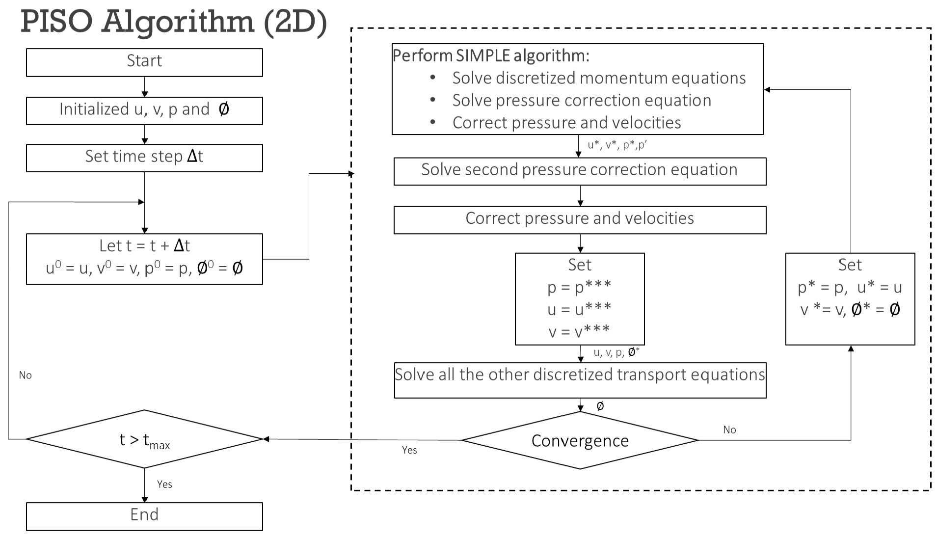
Several solver procedures available in the OpenFOAM, with PISO (Pressure Implicit with Splitting of Operators), were originally used (Kissling et al., 2010). PISO (Iissa et al., 1986) is a pressure-velocity calculation procedure originally developed for unsteady compressible flows with involves one predictor step and two corrector steps. A new algorithm of PIMPLE has been developed, which is the mixture between PISO and SIMPLE (Semi-implicit Method for Pressure-linked Equations). SIMPLE originally introduced by Patankar and Spalding (1972) is essentially a guess-and-correct procedure for calculating the pressure on the staggered grid. The $p^{*}$ is guessed and used to yield the components $u^{*}, v^{*}$ , and $w^{*}$ then correct the pressure and velocities. PISO, SIMPLE and PIMPLE methods are used for pressure-velocity coupling (momentum and continuity equations will be solved together). The original PISO solving algorithm which is extended from SIMPLE with an additional corrector step can be seen in Fig. 1. OpenFOAM utilized the FVM.

https://cdn.apub.kr/journalsite/sites/kwra/2023-056-12S/N020056S-106/images/kwra_56_S-1_06_F1.jpg

Fig. 1.

Flowchart for solving PISO algorithm

2.5 Model setup

2.5.1 Simulation Scenarios

The comparative study of the laminar and RANS turbulence model will be assessed by using two dam-break flow scenarios around the structure. The two simulated scenarios consist of:

1) Dam-break flow against an isolated obstacle (Soares-Frazão and Zech, 2007).

2) Dam-break flow against a multi-layered obstacle (modified from the first scenario).

An experiment conducted by Soares-Frazão and Zech (2007) has yielded relatively high-quality datasets and has been adopted extensively to validate the numerical modeling. The second scenario was developed to be able to capture significant differences in laminar and turbulence flow characteristics around multi-layered structures.

2.5.2 Mesh generation

OpenFOAM provides several features for mesh generation tools such as “BlockMesh” and “SnappyHexMesh”. In this study, both tools were utilized to create the simulation domain and structure generation. Moreover, gate opening was set in the experimental set-up by Soares-Frazao. Therefore, another tool of mesh generation, “TopoSet” was used to create the gate opening at the model set-up. An additional third-party application (FreeCAD) was also applied in this study to generate the structure (single obstacle and multi-layered obstacle), then generated in the numerical domain by utilizing the “SnappyHexMesh” within the OpenFOAM.

The computational domain was designed following the water tank dimension within the experiment set-up in the reference, with an almost 36 m length and 3.6 m width. The reservoir was designed with a 1 m opening located at 6.9 m from the upstream. Hexahedral grids selected in this domain with finer grid sizes used for both simulations to maintain the stability. The numerical grid set-up and corresponding time step for both scenarios are shown in Table 1. Initial timestep was user-defined, however, the timestep will be adjusting based on the model stability by maintaining the CFL (Courant-Friedrichs-Lewy) number.

Table 1.

Mesh generation set-up

Parameter	Laminar	RANS
Cell number	900,000	900,000
Timestep	0.01	0.01
Adjustable	yes	yes

2.5.3 Initial and boundary conditions

The initial condition of this model consists of water with 0.4 m height in the reservoir and a thin layer of 0.02 water in the channel to ensure the nonslip condition. The gate opening is controlled to be instantaneously opened. The initial water level is generated by the built-in function in the OpenFOAM to fill the cells with water using “SetFields” tools. The function sets the VOF function with 0 or 1 defining the cells filled with water. We incorporate the gate opening by creating water behind the dam as a column of water at rest located behind a membrane. When the gate opens at time t = 0 s, the membrane is removed resulting in the column of water collapsing.

The upstream boundary conditions in the simulation domain are specified as ‘walls’ (Fig. 2(a)) with defined no flow entering the domain. The top boundary is employed as the atmospheric pressure with “totalPressure”. The side of the channel is specified as walls with assumed as no-slip condition, while zero velocity is specified in the obstacle. The logarithmic velocity profile distribution in the wall function is applied by RANS to calculate the shear stress incorporating the turbulence closure model. Detailed wall function and boundary condition specified in the model can be seen in Table 2.

https://cdn.apub.kr/journalsite/sites/kwra/2023-056-12S/N020056S-106/images/kwra_56_S-1_06_F2.jpg

Fig. 2.

Numerical domain (a) Scenario 1: Dam-break flow over the isolated obstacle; (b) Scenario 2: Dam-break flow over the multi-layered obstacle

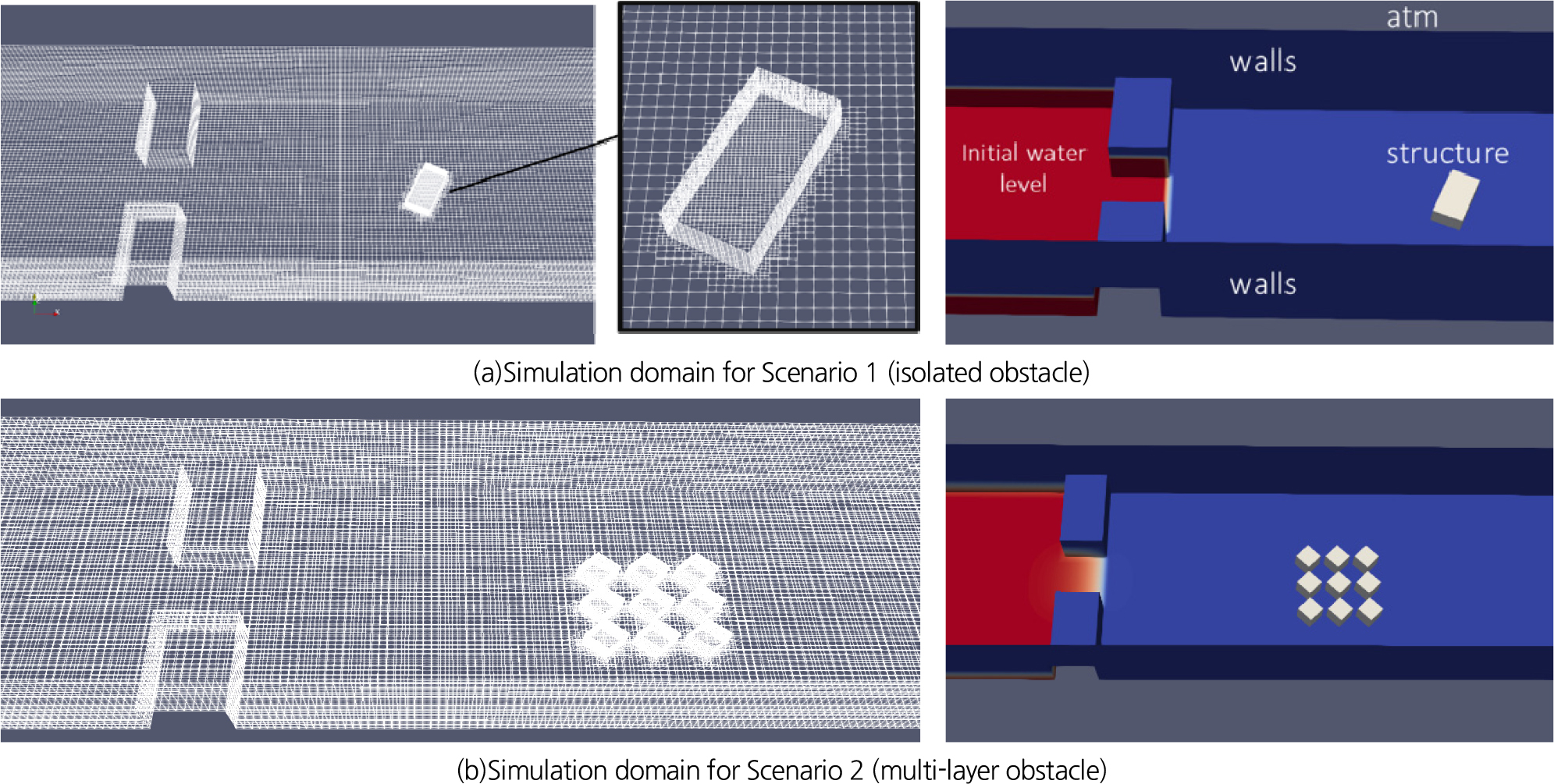
Table 2.

Numerical schemes and solving procedures specified in the model

Laminar Model		RANS Model
ddtSchemes	Euler	ddtSchemes	Euler
gradSchemes	Gauss Linear	gradSchemes	Gauss Linear
div(rhoPhi,U)	Gauss linearUpwind grad (U)	div(rhoPhi,U)	Gauss linearUpwind grad(U)
div(phi,alpha)	Gauss vanLeer	div(phi,alpha)	Gauss vanLeer
div(phirb,alpha)	Gauss linear	div(phirb,alpha)	Gauss linear
		div(rhoPhi,k)	Gauss upwind
		div(rhoPhi,epsilon)	Gauss upwind
		div(((rhonuEff)dev2(T(grad(U)))))	Gauss linear;
laplacianSchemes	Gauss linear orthogonal	laplacianSchemes	Gauss linear orthogonal
Laplacian(nu,U)		Laplacian(DkEff,k)
		Laplacian(DepsilonEff,epsilon)
Solving procedure	PISO	Solving Procedure	PIMPLE (PISO + SIMPLE)

2.5.4 Numerical scheme and solving procedure

The discretization schemes specified in this model are represented for each term of the governing equation. The selected schemes follow the original schemes proposed by Jasak (1996), with the Euler scheme for time discretization and Gauss linear (central difference) and the upwind scheme selected for spatial discretization. The additional turbulence closure terms were added in the RANS model.

The original PISO solving algorithm will be used in the laminar simulation, while the PIMPLE solving algorithm used for the RANS simulation to ensure stability. The keywords “nOuterCorrectors” are added to activate the PIMPLE loop which allows the re-calculation of pressure and momentum coupling. The keywords “nNonOrthogonal Correctors” and “relaxationFactors” are added to complete the PIMPLE mode and activate the SIMPLE calculation and pressure field correction due to the non-orthogonal meshes.

3. Numerical Results

3.1 Scenario 1 - Isolated obstacle

The simulation result from both the laminar and RANS model compared with the experimental data conducted by Soares and Frazao (2007). The velocity and water depth profile can be seen in Figs. 3 and 4. The observation point selected for the comparison is located in front of the obstacle (G2), the right (G3) and left (G4) side of the obstacle, and behind the obstacle (G5). The significant difference in the laminar model is the spurious water profile due to the absence of the turbulence closure. The laminar model shows a high instability, especially in the early stage of simulation in front of the obstacle. Generally, both laminar and RANS shows adequately represent the velocity profile compared to the experimental setup. The numerical dissipation effect in the RANS model dominantly affects the numerical result although in some cases it shows underestimated results due to the extensive turbulence dissipation.

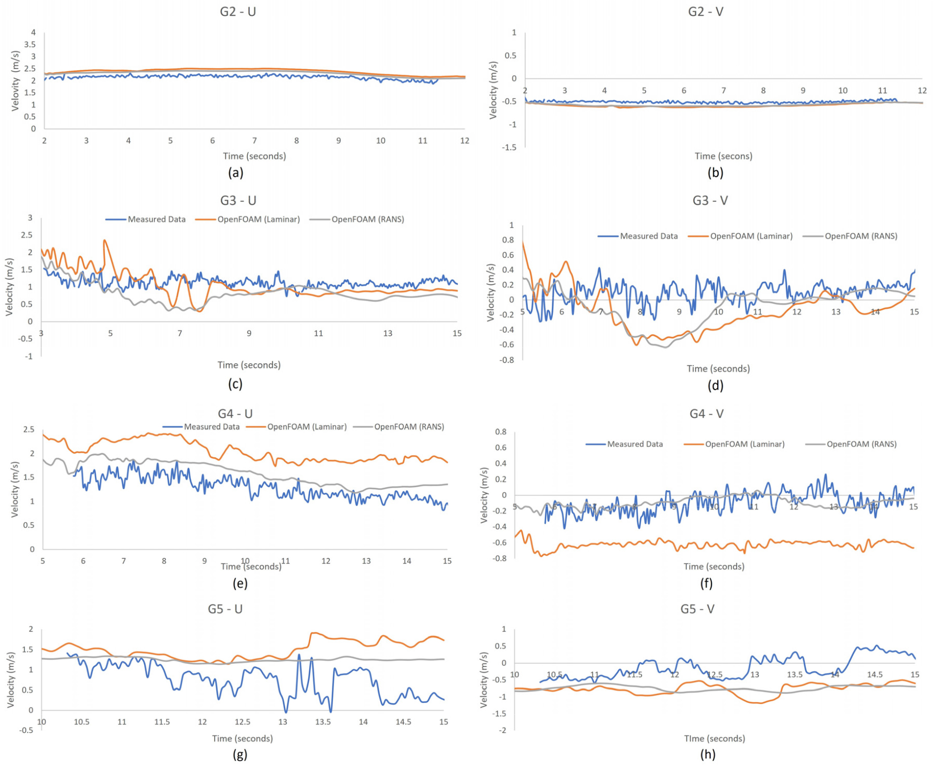
https://cdn.apub.kr/journalsite/sites/kwra/2023-056-12S/N020056S-106/images/kwra_56_S-1_06_F3.jpg

Fig. 3.

Velocity profile of simulated scenario 1 compared with experiment data from (Soares-Frazão and Zech, 2007)

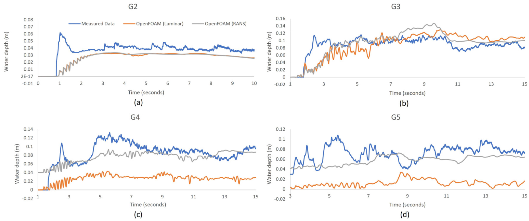
https://cdn.apub.kr/journalsite/sites/kwra/2023-056-12S/N020056S-106/images/kwra_56_S-1_06_F4.jpg

Fig. 4.

Water depth profile of simulated scenario 1 compared with experiment data from (Soares-Frazão and Zech, 2007)

The formation of the hydraulic jump causes a high oscillation in the laminar model. The laminar model shows instability along the simulation in every observation point location. The dam-break flow exhibits heightened turbulence, particularly as it develops near the wavefront, influencing both propagation and flow dynamics around obstacles. The RANS simulation only shows better prediction compared to the laminar model at several locations, especially after 5 seconds. This outperformance is due to the RANS k-ε model being established based on the time-averaging of the mean and fluctuating process, while the discontinuity and unsteadiness of the dam-break profile are quite prominent.

3.2 Scenario 2 - Multi-layered obstacles

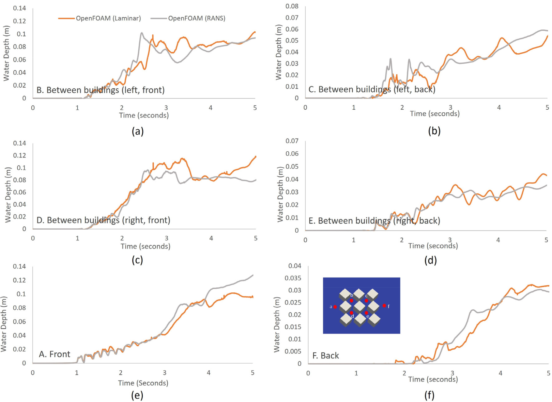
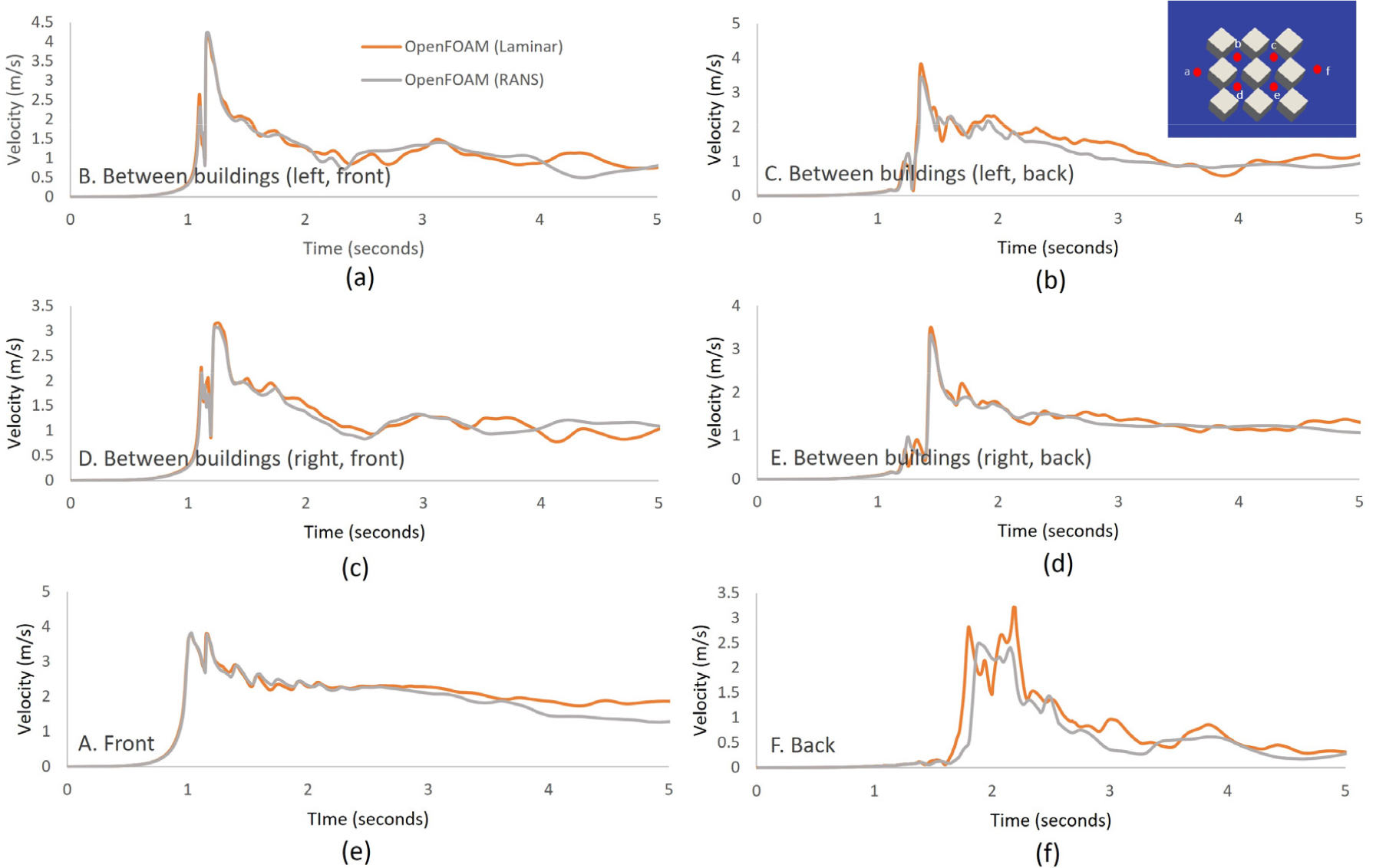
The comparison of the laminar and RANS models in scenario 2 can be seen in Figs. 5 and 6. The objective of this simulation is to obtain a clear and significant difference between the laminar and turbulent models, since the turbulent closure is more dominant and able to accurately describe the dam-break flow in the complex topography. The observation points are located at 6 different locations, i.e., (a) located in front of the obstacle, (b, d) between the obstacle in the first layer building, (c, e) second layer of building and (f) behind the building. The water depth profile in front of the obstacle shows a similar pattern with scenario 1, with a high oscillation for the laminar model. This shows that the laminar model is incapable of simulating the dam-break wavefront profile. The RANS model shows its capability in simulating the flow profile with a smooth free surface without any spurious oscillation during the abrupt change of topography due to the obstacle. The velocity profile in the RANS simulation shows the peak velocity to occur earlier compared to the laminar flow, although the difference of peak time is relatively small (less than seconds). This phenomenon may result due to the better performance of the RANS model in predicting the wave front water depth and celerity.

https://cdn.apub.kr/journalsite/sites/kwra/2023-056-12S/N020056S-106/images/kwra_56_S-1_06_F5.jpg

Fig. 5.

Water depth profile of simulated scenario 2

https://cdn.apub.kr/journalsite/sites/kwra/2023-056-12S/N020056S-106/images/kwra_56_S-1_06_F6.jpg

Fig. 6.

Velocity profile of simulated scenario 2

4. Discussion

Based on the two scenarios simulated in this study, the significant difference in the dam-break flows simulated using the laminar and RANS model are represented in more detailed in this section. The discussion is divided based on the numerical schemes and solving procedure, model setup and governing equations.

4.1 Numerical schemes and solving procedure

The complete PIMPLE algorithm utilized in the RANS simulation increased the convergence rate which can be seen in the increase of numerical stability. However, the PIMPLE algorithm adds a solving procedure of momentum-pressure coupling which will eventually increase the simulation time based on the number of corrections setup. In the laminar simulation using the PISO algorithm, the number of corrections is added with a low number of iterations. Although the result shows high instability, the PISO mode re-calculated the pressure to avoid model errors.

4.2 Model set-up

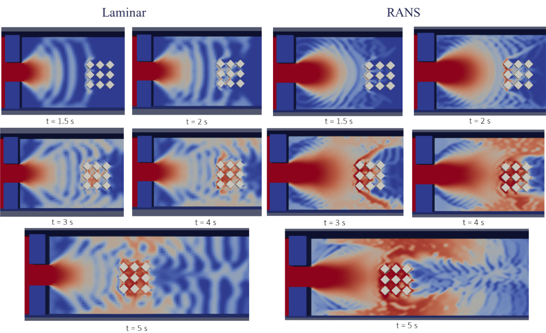
The finer grid significantly affects the flow profile especially in the turbulence flow, wake profile clearly represented behind the structure. The multiphase flow (VOF) is appropriate to include in the dam-break flow due to the sharp interface of water and air during the flow. The sharp interface of water and air clearly defined in the refined grid as can be seen in Fig. 7.

https://cdn.apub.kr/journalsite/sites/kwra/2023-056-12S/N020056S-106/images/kwra_56_S-1_06_F7.jpg

Fig. 7.

Flow profile simulation result of scenario 2: (left) Laminar model; (right) RANS model

4.3 Laminar and RANS model

Both models show a good capability to represent the dam-break flow. The RANS model adequately represented the depth profile in the early stage especially in predicting the wavefront propagation and flow interaction in complex topography (between obstacles). The laminar simulation produces a spurious water profile due to the lack of turbulence dissipation. However, the RANS simulation only shows a slightly improved performance due to the time-averaging base for solving the turbulence properties. RANS simulation shows underestimated results due to the extensive turbulence dissipation. The turbulence dissipation contributed to reducing the numerical oscillation and increasing model stability.

5. Conclusion

Both the laminar and RANS models show a good capability to represent the dam-break flow. The turbulence closure using RANS (k-ε model) simulations reduces the oscillation in the model by adding the turbulent dissipation. However, the extensive dissipation may result in an underestimated water profile. Improving the numerical scheme and finer grid have a significant impact on recreating the dam-break flow especially near the structure and improving the sharp interface of water and air especially during turbulence.

The application of improved numerical scheme and finer grid size may have a more significant impact on increasing the model stability compared to using the RANS model. This is due to the k-ε model being established based on the time-averaging of the mean and fluctuating process, while the discontinuity and unsteadiness of the dam-break profile are quite prominent. Moreover, the computational effort in simulating the turbulence model is relatively more extensive while the RNAS model only slightly improved the performance compared to the laminal model. To achieve the best representation of the dam-break flow, employing advanced turbulence models like LES and DNS is essential. Nevertheless, dealing with very small spatial and temporal scales required for this purpose remains a challenge, adding complexity to this subject. This challenge can be addressed by implementing a stable yet precise numerical scheme (Hwang and Son, 2023).

Acknowledgements

This work was supported by the National Research Foundation of Korea (NRF) grant funded by the Korea government (MSIT)(NRF-2019R1A2C1089109). This work was also supported by Korea Environment Industry & Technology Institute (KEITI) through R&D Program for Innovative Flood Protection Technologies against Climate Crisis Program (or Project), funded by Korea Ministry of Environment (MOE)(RS-2023-00218873).

Conflicts of Interest

The authors declare no conflict of interest.

References

Aureli, F., Dazzi, A., Maranzoni, A., Mignosa, P., and Vacondio, R. (2015). "Experimental and numerical evaluation of the force due to the impact of a dam break wave on a structure." Advance Water Resources, Vol. 76, pp. 29-42. 10.1016/j.advwatres.2014.11.009

Biscarini, C., Francesco, S.D., and Manciola, P. (2010). "CFD modelling approach for dam break flow studies." Hydrology and Earth System Sciences, Vol. 14, No. 4, pp. 705-718. 10.5194/hess-14-705-2010

Chanson, H. (2006). "Tsunami surges on dry coastal plains: Application of dam break wave equations." Coastal Engineering Journal, Vol. 48, No. 4, pp. 355-370. 10.1142/S0578563406001477

Delisle, M.-P.C., Kim, Y., and Gallien, T.W. (2023). "A numerical study of dam-break driven swash and beach groundwater interactions." Journal of Geophysical Research: Oceans, Vol. 128, No. 9, e2022JC019615. doi: 10.1029/2022JC019615. 10.1029/2022JC019615

Evangelista, S. (2015). "Experiments and numerical simulations of dike erosion due to a wave impact." Water, Vol. 7, pp. 5831-5848. 10.3390/w7105831

Hien, L.T.T., and Van Chien, N. (2021). "Investigate impact force of dam-break flow against structures by both 2D and 3D numerical simulations." Water, Vol. 13, No. 3, 344. doi: 10. 3390/w13030344. 10.3390/w13030344

Higuera, P., Lara, J.L., and Losada, I.J. (2013). "Simulating coastal engineering processes with OpenFOAM®." Coastal Engineering, Vol. 71, pp. 119-134. doi: 10.1016/j.coastaleng.2012. 06.002. 10.1016/j.coastaleng.2012.06.002

Hwang, S., and Son, S. (2023). "An efficient HLL-based scheme for capturing contact-discontinuity in scalar transport by shallow water flow." Communications in Nonlinear Science and Numerical Simulation, Vol. 127, 107531. 10.1016/j.cnsns.2023.107531

Iissa, R., Gosman, A.D., and Watkins, A.P.(1986). "The computation of compressible and incompressible recirculating flows by a non-iterative implicit scheme." Journal of Computational Physics, Vol. 62, No. 1, pp. 66-82. 10.1016/0021-9991(86)90100-2

Jasak, H. (1996). Error analysis and estimation for the finite volume method with applications to fluid flows. Ph.D. Thesis, Imperial College of Science, London, UK.

Kim, Y., Zhou, Z., Hsu, T.-J., and Puleo, J.A. (2017). "Large eddy simulation of dam-break-driven swash on a rough-planar beach." Journal of Geophysical Research: Oceans, Vol. 122, pp. 1274-1296, doi: 10.1002/2016JC012366. 10.1002/2016JC012366

Kissling, K., Springer, J., Jasak, H., Schutz, S., Urban, K., and Piesche, M. (2010). "A coupled pressure based solution algorithm based on the volume-of-fluid approach for two or more immiscible fluids." V European Conference on Computational Fluid Dynamics, ECCOMAS, Lisbon, Portugal, pp. 1-16.

Kocaman, S., Güzel, H., Evangelista, S., Ozmen-Cagatay, H., and Viccione, G. (2020). "Experimental and numerical analysis of a dam-break flow through different contraction geometries of the channel." Water, Vol. 12, No. 4, 1124. doi: 10.3390/ w12041124. 10.3390/w12041124

Launder, B.E., and Spalding, D.B. (1974). "The numerical computation of turbulent flows." Computer Methods in Applied Mechanics and Engineering, Vol. 3, No. 2, pp. 269-289. 10.1016/0045-7825(74)90029-2

Liu, D., Tang, W., Wang, J., Xue, H., and Wang, K. (2016). "Comparison of laminar model, RANS, LES and VLES for simulation of liquid sloshing." Applied Ocean Research, Vol. 59, pp. 638-649. doi: 10.1016/j.apor.2016.07.012. 10.1016/j.apor.2016.07.012

Patankar, S.V., and Spalding, D.B. (1972). "A calculation procedure for heat, mass and momentum transfer in three-dimensional parabolic flows." International Journal of Heat Mass Transfer, Vol. IS, pp. 1787-1806. 10.1016/0017-9310(72)90054-3

Robb, D.M., and Vasquez, J.A. (2015). "Numerical simulation of dam-break flows using depth-averaged hydrodynamic and three-dimensional CFD Models." 22nd Canadian Hydrotechnical Conference, CSCE, Nontreal, Canada, pp. 27-36.

Rodríguez-Ocampo, P.E., Ring, M., Hernández-Fontes, J.V., Alcérreca-Huerta, J.C., Mendoza, E., and Silva, R. (2020). "CFD simulations of multiphase flows: Interaction of miscible liquids with different temperatures." Water, Vol. 12, No. 9, 2581. doi: 10.3390/w12092581. 10.3390/w12092581

Rusche, H. (2002). Computational fluid dynamics of dispersed two-phase flows at high phase fractions. Ph.D. Thesis, Imperial College of Science, London, UK.

Soares-Frazão, S. (2007). "Experiments of dam-break wave over a triangular bottom sill." Journal of Hydraulic Research, Vol. 45, No. sup1, pp. 19-26. 10.1080/00221686.2007.9521829

Soares-Frazão, S., and Zech, Y. (2002). "Dam Break in channels with 90^o bend." Journal of Hydraulic Engineering-ASCE, Vol. 128, No. 11, pp. 956-968. 10.1061/(ASCE)0733-9429(2002)128:11(956)

Soares-Frazão, S., and Zech, Y. (2007). "Experimental study of dam-break flow against an isolated obstacle." Journal of Hydraulic Research, Vol. 45, No. sup1, pp. 27-36. 10.1080/00221686.2007.9521830

Journal of Korea Water Resources Association ISSN:2799-8746(Print) 2799-8754(Online) 한국수자원학회 논문집

Preview

Comparative study of laminar and turbulent models for three-dimensional simulation of dam-break flow interacting with multiarray block obstacles

ABSTRACT

MAIN

(1)

(2)

(3)

(4)

(5)

(6)

(7)

(8)

(9)

(10)

(11)

(12)

(13)

(14)

(15)

Fig. 1.

Flowchart for solving PISO algorithm

Table 1.

Mesh generation set-up

Fig. 2.

Numerical domain (a) Scenario 1: Dam-break flow over the isolated obstacle; (b) Scenario 2: Dam-break flow over the multi-layered obstacle

Table 2.

Numerical schemes and solving procedures specified in the model

Fig. 3.

Velocity profile of simulated scenario 1 compared with experiment data from (Soares-Frazão and Zech, 2007)

Fig. 4.

Water depth profile of simulated scenario 1 compared with experiment data from (Soares-Frazão and Zech, 2007)

Fig. 5.

Water depth profile of simulated scenario 2

Fig. 6.

Velocity profile of simulated scenario 2

Fig. 7.

Flow profile simulation result of scenario 2: (left) Laminar model; (right) RANS model

Acknowledgements

Conflicts of Interest

References