

I. Introduction
Groundwater is an important reservoir of water with various applications. Currently, there are many risks in terms of water pollution as a result of development of industries, population growth, and lack of proper environmental control. Therefore, necessary planning can be made to make the best use of water resources in a country by recognizing qualitative characteristics of water. Being aware of water quality is one of the important requirements for planning and developing water resources together by protecting and controlling them. Obviously, monitoring and evaluating are necessary in order to generate the required information and be aware of the quality of water resources, because having comprehensive and accurate information in appropriate periods can be considered as an important factor for decision and policy-making. Groundwater is one of the most major sources of fresh water in all areas, and in dry and semi-arid areas of the world, it is the only source of water. Due to its easy accessibility, groundwater is still regarded as the principal supply even in regions with favorable rainfall circumstances. (Mohtashami et al., 2021) Changes in groundwater quality that usually occur because of mismanagement of groundwater use are a basis for the destruction of water resources and other resources both directly and indirectly. In arid and semi-arid regions, which are more dependent on these resources, the destructive effect will be more severe due to natural weakness in water and soil resources. Therefore, the need to study and evaluate its quality in Iran can be helpful for properly managing the use of water resources (Zehtabian et al., 2010). In this study, referring to (Azimi et al., 2018a) as the most significant factor, in water quality variation in aquifers, the relationship between climatic drought effects on groundwater resources was studied. By using Gaussian process classification and back propagation artificial neural network, the association analysis of climate draught and a reduction in groundwater quality was implemented. Underground water level in 609 study areas in Iran was used to anticipate drought over the test period extending. In recent years, supplying the required water for drinking, industry, and agricultural purposes has faced problems in many countries due to improper use, entry of industrial and chemical pollutants, and the reduced quality of water resources (Dagostino et al., 1998). Knowing the state of a region's water resources is crucial for water planning and agriculture. Thus, urban and rural populations must be informed of the future state of water resources, particularly in standard drinking water classes (Eberhard and Hamawand, 2017), (Azimi et al., 2018b). There are various methods for studying and zoning changes in surface and groundwater characteristics, each of which has different levels of accuracy depending on conditions of the region and the existence of sufficient statistics and data (Soleimani et al., 2012). It is of high importance to study spatial and temporal alterations in water quality parameters and to know qualitative status of surface water and groundwater and also to determine the most proper management strategy in order to develop the quality of water resources (Osati et al., 2013). On a general basis, a review of research records associated with the study topic demonstrates that generally, monitoring and assessing quality of water resources is a relatively new activity but is currently expanding rapidly. Although, using Geographic Information System (GIS) has made considerable progress and development in water quality studies, a number of problems and challenges have remained to be solved regarding the data set used in national, regional, zonal, and local studies; highlighting the need for carrying out some studies to solve such problems. In this study, the best water quality zoning was done with the minimum error using GIS, and by forming a very regular and analytical database for managing qualitative trend of surface and groundwater over the past 30 years and analyzing this database with a variety of qualitative methods and combining them. In India, (Balakrishnan et al., 2011) prepared and interpreted groundwater quality maps using GIS software. (Jamshidzadeh et al., 2011a) conducted studies on quality of an aquifer in the central plain of Iran, zoned and mapped quality parameters by GIS software, and found that most samples are not suitable for drinking water. (Samin et al., 2012) used Kriging and Co-Kriging methods to estimate ratio of sodium and chlorine uptake in groundwater of 90 wells in Fars Province and concluded that estimates of both methods are acceptable but accuracy of Co-kriging method is higher than Kriging one in estimating sodium and chlorine uptake. (Azizi and Mohammadzadeh, 2012) used groundwater quality index (GWQI) to study water quality of Imamzadeh Jafar Plain in Gachsaran and compared it by Schuler method. They showed that about 2, 83, and 12% of the groundwater resources in Imamzadeh Jafar Plain are of excellent, good, and bad quality, respectively. (Shabani, 2009) through comparing different interpolation methods to map changes in pH and total dissolved solids (TDS) of groundwater in Arsanjan Plain concluded that simple and ordinary Kriging method are superior to other methods. (Delgado et al., 2010) collected 113 water samples from wells in the Yucatan Plain in Mexico. Concentrations of calcium, magnesium, sodium, potassium, bicarbonate, sulfate, nitrate, and chlorine ions and electrical conductivity (EC) were determined and ratio of sodium absorption, potential salinity, and effective salinity were calculated and the region was divided into 6 sub-regions in terms of water quality. The results reveal that the groundwater resources in areas 1, 2, and 3 were at risk of salinity and unusable for agricultural purposes. (Adhikary et al., 2011) used the geostatistical method for determining quality of groundwater and assessing risk of groundwater pollution in Najaf Gare Plain in India and after preparing thematic maps of quality parameters of groundwater, such as bicarbonate, calcium, EC, magnesium, nitrate, sulfate, and sodium, they concluded that the Kriging method was appropriate for assessing risk of groundwater contamination. (Hooshmand et al., 2011) used geostatistical tools, like Kriging and Co-kriging to simulate variables of groundwater quality. The results indicated that the Co-kriging method is better than other geostatistical tools for simulating variables of groundwater quality. In a study, (Adhikary et al., 2012) investigated quality of groundwater in the suburbs of Delhi, India for irrigation and drinking purposes using GIS and Geostatistics. In this research, ordinary Kriging method was applied to prepare thematic maps of water quality parameters including HCO, sodium absorption ratio (SAR), EC, Mg to Cl ratio, TDS, Ca, nitrate, and water hardness. The spherical variogram model indicated the best fit to the data for two qualitative parameters including Cl and water hardness; and in other cases, the best fit was indicated by the exponential model. Distribution maps of quality index of irrigation water and drinking water showed that areas of 47.29 and 6.54 square kilometers were suitable for irrigation and drinking purposes. While (Khomr et al., 2011) through studying quality of water resources in the Kuh Zar mineral area in west of Torbat-e-Heydarieh, which was based on the Wilcox diagram indicated that water quality of that region is unsuitable for agricultural use. (Soleimani et al., 2012) in a study on evaluating efficiency of geostatistical methods for preparing a map of changes in pH and TDS of springs in the Mire Catchment area in Kurdistan found that using general grade 3 polynomial interpolation maps and simple Kriging, one is able to estimate TDS and pH values of springs in the catchment area, respectively. (Gebrehiwot et al., 2011) used water quality index (WQI) method to study groundwater quality of the northern Ethiopian aquifer for drinking purposes and investigated water quality of the area using ten qualitative parameters including Mg, Na, K, Ca, Cl, SO4, HCO3, TDS, EC, and pH and found that WQI variation was between 54 - 86%, and all samples were of decent quality. The purpose of this research is to investigate trend of groundwater quality over 25 years and prepare the combined zoning for estimating quality parameters applying common standards, analyzing, and interpreting them with minimum error and uncertainty. Because such a study has not been conducted to investigate various dimensions of qualitative parameters in all aquifers, performing the current research appears to be necessary in this field.
II. Materials and Methods
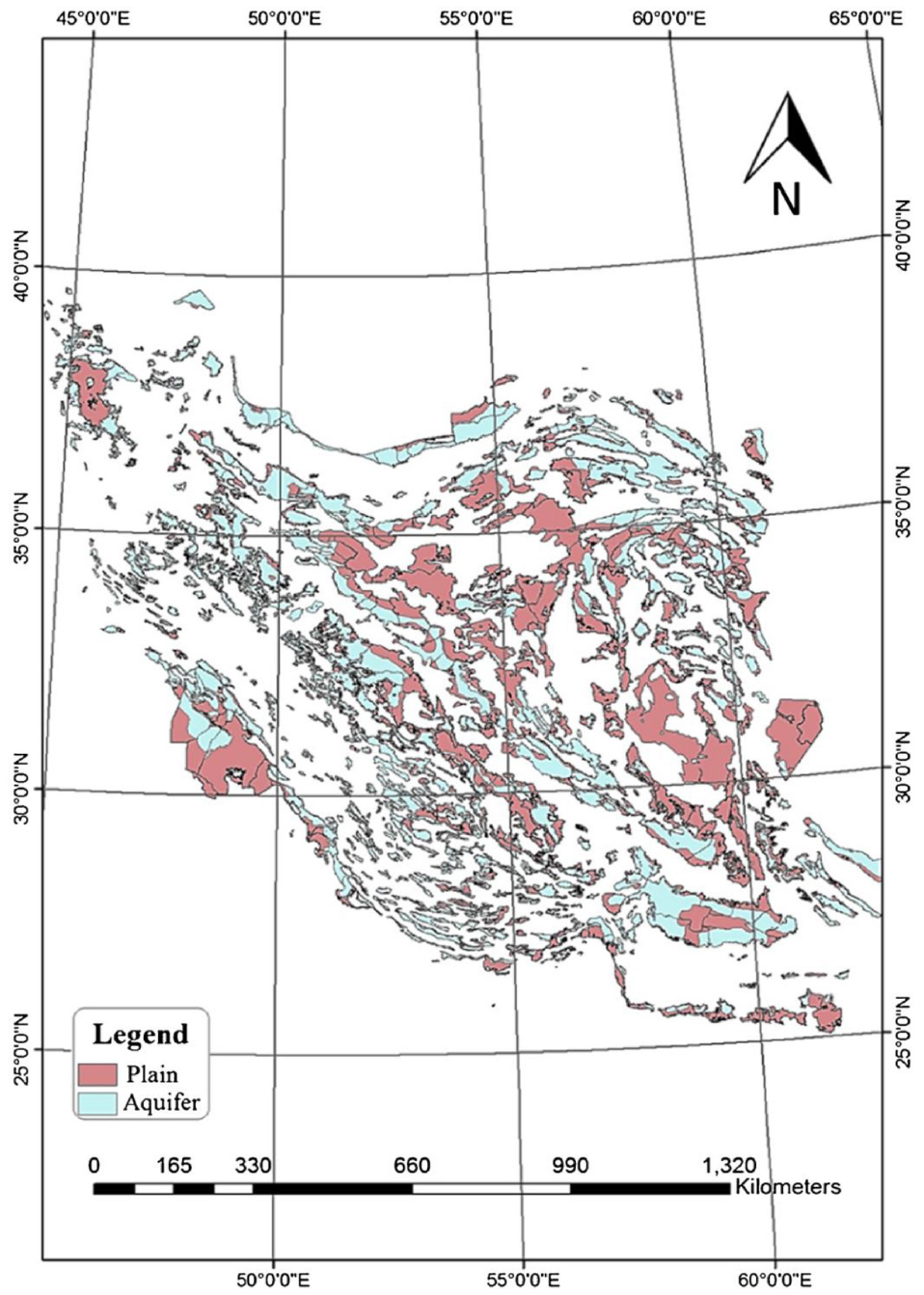
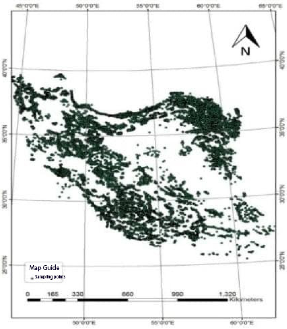
The study area is in the boundary of Iran, and zoning was done according to vector-layer of the plains. Fig. 1 shows location of the plains of Iran along with location of aquifers. The geographical system used in this study was WGS1384, and for creating computational conditions, the status for collecting the point data of wells was converted from the original form of universal transverse Mercator (UTM) into decimal form using four zones of 38, 39, 40, and 41. Due to unavailability of the initial value, the method for calculating zone was based on station number and its correspondence with the plain number. For the points located in border plains, format differentiation and numerical structure of their depicted coordinates were used in order to identify and separate them. Fig. 2 indicates position of four zones of Iran as well as position of sampling wells after converting the coordinates.
The statistical period was considered from 1995 to 2020 in two 12-year categories in the same period as well. According to the number of 12 millions, quality data of the groundwater resources of Iran were tested by elimination validation methods. This method is based on determining confidence interval using distribution characteristics of statistical data. The type of variables҆ probability density distribution function was determined based on the available data, and if the data were outside the calculated confidence interval with respect to the desired confidence level, they were re-assessed as suspicious data and were deleted if the error was confirmed. Then, using inverse validation, compatibility between qualitative variables was investigated according to their characteristics. Therefore, a series of specific relationships were defined for physical, chemical, and biological variables of water quality by which the mentioned variables were controlled and if a relationship was not true, the issue was validated and deleted (Karamouz and Karachian, 2008). After verifying the data and before performing statistical calculations and analyses, it should be ensured that there is no non-random pattern in the data. Among the proposed patterns, trend is very important. In this regard, nature of the basic parameters was investigated. For this purpose, random trend in the data was investigated through addition of geostatistical analyses in the GIS environment. The results of these studies indicated the existence of a quadratic trend in direction of north to south and east to west in all parameters. Additionally, in a detailed test called Run chart in Minitab software environment, for confirming accuracy of visual result of the trend in the basic parameters҆ data, the presence of trend was confirmed at least in two out of four checking conditions. In this case, if the P-Value is less than 5%-threshold, then the null hypothesis will be rejected, indicating that there is no trend. Since, distribution of some columns of available data did not follow normal distribution, and because many statistical calculations are based on the assumption that the data are normal and random, data distribution of all stations became normal step-by-step by choosing the most appropriate method among the methods of normalization equations including BOX-COX-Johnson-Transformation. Two basic methods are possible for addition of geostatistical analyses in GIS environment herein; logarithmization was used to normalize the data. For checking static status of the data, as another basic condition for creating zoning maps, the data mean was tested in unpaired categories using Minitab statistical software. In any case, where the assumption of static data is rejected, we will not be allowed to use ordinary and simple Kriging methods. In this study, due to practical use of data means in the categories of 10 and 20 years, the assumption of static data can be practically ignored. The results of testing the mean hypothesis indicated the lack of static status in data in all parameters, attributing to long statistical period and the trend of their downward and upward changes. After performing the statistical methods, the zoning maps were developed using a combination of geostatistical analyses in the GIS environment, based on inverse distance weighting (IDW), radial basic function (RBF), and global polynomial interpolation (GPI) methods, as well as Kriging and Co-kriging geostatistical methods in three types of simple, ordinary, and universal. Then, the maps generated in each parametric category were compared using the criteria of mean error (Mean), root mean square error (RMSE), mean squared (MS), root mean square error standardized (RMSES), and average standard error (ASE). Finally, the least uncertainty and the least zoning error were selected with respect to the criterion of being near zero for all errors and close to one for RMSES index in addition to proximity of two values of ASE and RMSE. Details regarding the error values for these methods are given in Table 1. In addition, the time series correlation of the basic variables was calculated in pairs in order to develop the Co-kriging method using the detection coefficient.
Table 1.
Error value of the interpolation methods for parameters
Methods, such as simple Kriging, simple Kriging, ordinary Kriging, ordinary Kriging, ordinary Kriging, ordinary Kriging, simple Kriging, ordinary Kriging, ordinary Co-kriging, ordinary Co-kriging, ordinary Kriging, simple Kriging, RBF, ordinary Kriging ,and simple Kriging were selected as the most optimal zoning by comparing the error generated with the computational and observational figures in the place of samples, for the parameters including HCO3-, CL-, SO42-, pH, EC, TDS, TH, SAR, Na%, K, Na+, Mg2+, +Ca2, and CO3, respectively. The best variogram was the variogram of the fitted model on experimental variogram of the parameters in each of the selected interpolation methods, with the exception of Mg parameter, which was interpolated by the RBF method.
A multiplicity of of data and their wide distribution in the geographical area of the study led to optimization of the maximum variogram of the model. Given the natural discontinuity of spatial variations in parameters from one aquifer to another, and due to simultaneous data analysis of all plains, for avoiding computational distortion, interpolation search window in all samples was reduced in a minimum number and a minimum distance with four sectors. The adjunctive automatic optimization was used to adjust the zoning factors in geostatistical methods and Mg sample. Also, in each case, if the amount of error was high, it was reduced by trial and error and changing the main equations of variogram fitting. According to Table 2, optimal interpolation model was selected.
Table 2.
Parameters for optimal interpolation model of variables
For evaluating quality of agricultural water based on the Wilcox standard, a classification map was extracted in the mentioned three periods. According to the Wilcox diagram, water quality is divided into four classes. Table 3 indicates the limit and degree of quality of each class.
Table 3.
Wilcox index criteria in classification of agricultural water
| Quality type | EC | SAR |
| Excellent | <250 | <10 |
| Good | 250-750 | 10-18 |
| Average | 750-2250 | 18-26 |
| Unsuitable | >250 | >26 |
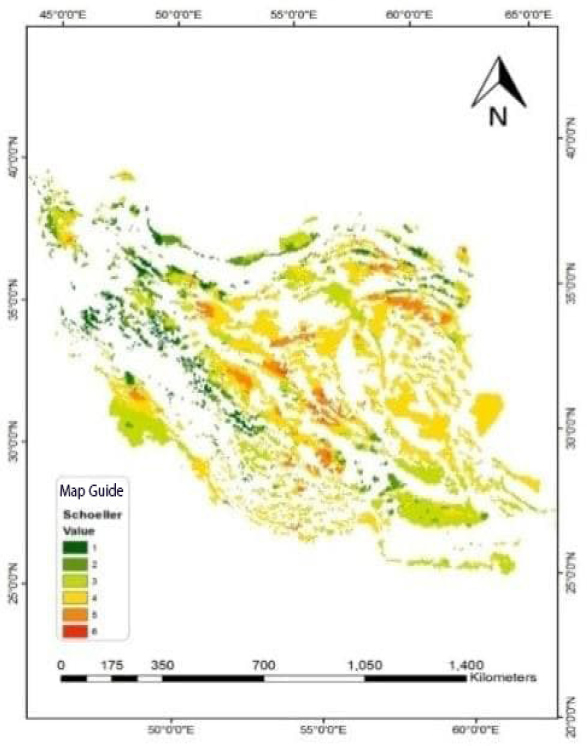
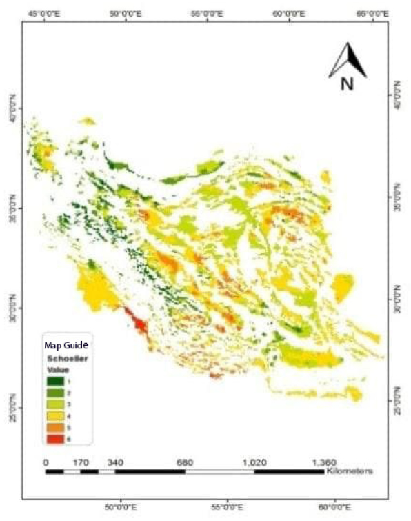
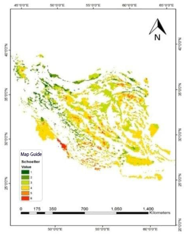
For evaluating quality of drinking water based on the Schuler standard, a classification map was extracted in the mentioned three periods. According to Schuler diagram, water quality is divided into six classes. Water quality classes, as well as limit of each of the six groups are listed in Table 4.
Babiker et al. (2007) in a study assessed groundwater quality using GWQI (Babiker et al., 2007) using which the parameters including TDS, Cl-, SO42-, Ca2+, Mg2+, and Na+ are integrated and spatial changes in groundwater quality are evaluated. The output results of this index will be presented in percentage, and the higher this value, the higher the water quality at that point is.
Table 4.
Schuler index criteria for classification of drinking water
III. Results and Discussion
Methods including simple Kriging, simple Kriging, ordinary Kriging, ordinary Kriging, ordinary Kriging, ordinary Kriging, simple Kriging, ordinary Kriging, ordinary Co-kriging, ordinary Co-kriging, ordinary Kriging, simple Kriging, RBF, ordinary Kriging, and simple Kriging were selected as the most optimal zoning by comparing the error generated with computational and observational figures in the place of samples, for the parameters including HCO3-, CL-, SO42-, pH, EC, TDS, TH, SAR, Na%, K, Na+, Mg2+, + Ca2, and CO3, respectively. Then, a combined model of each parameter was selected by coding in Python software, and zoning was performed based on Schuler, Wilcox, and GWQI indices. According to long-term changes in the model, a decrease in groundwater quality was observed. As shown in Figs. 3~6 the zoning was done with 12-year intervals by Wilcox index and combined interpolation method.
Methods including simple Kriging, simple Kriging, ordinary Kriging, ordinary Kriging, ordinary Kriging, ordinary Kriging, simple Kriging, ordinary Kriging, ordinary Co-kriging, ordinary Co-kriging, ordinary Kriging, simple Kriging, RBF, ordinary Kriging, and simple Kriging were selected as the most optimal zoning by comparing the error generated with computational and observational figures in the place of samples, for the parameters including HCO3-, CL-, SO42-, pH, EC, TDS, TH, SAR, Na%, K, Na+, Mg2+, +Ca2, and CO3, respectively. Then, a combined model of each parameter was selected by coding in Python software, and zoning was performed based on Schuler, Wilcox, and GWQI indices. According to long-term changes in the model, a decrease in groundwater quality was observed. As shown in Figs. 3~6 the zoning was done with 12-year intervals by Wilcox index and combined interpolation method.
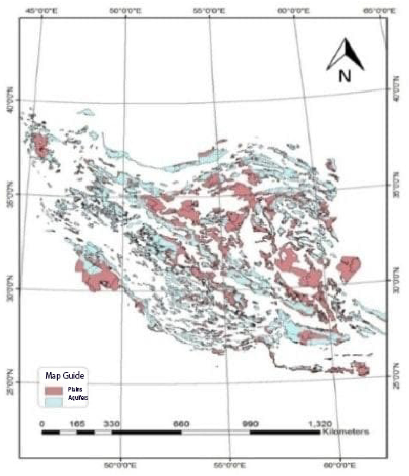
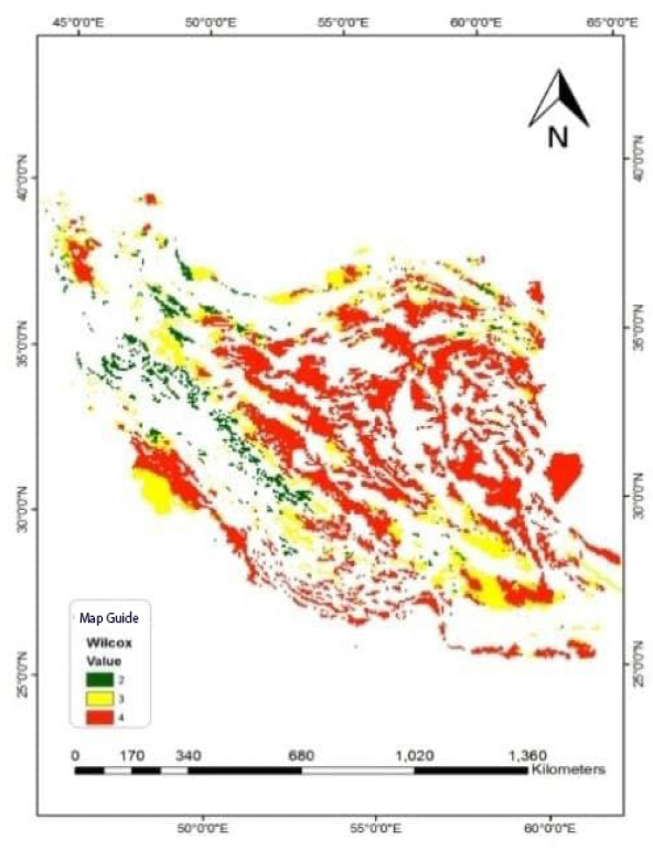

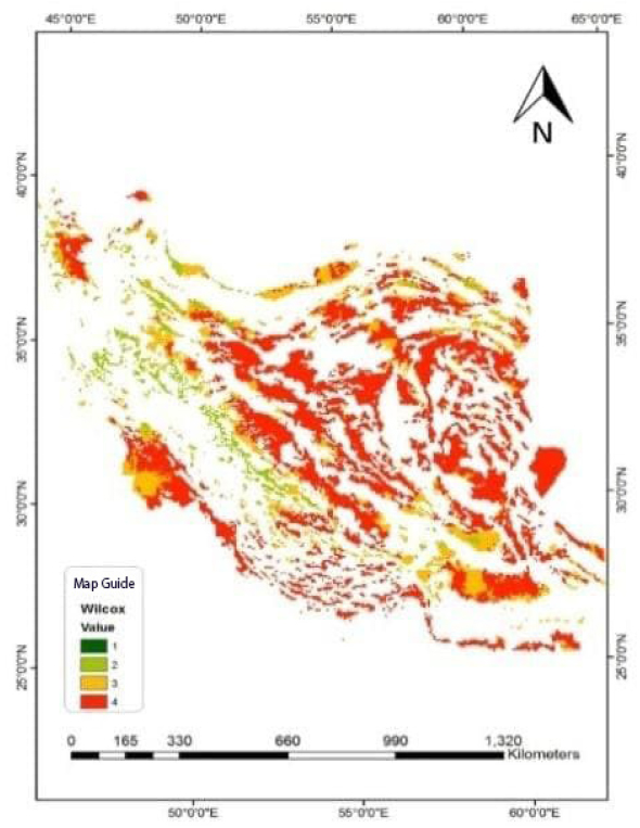
Table 5 indicates a statistical summary regarding percentage of quality classes of Wilcox index for agricultural water in Iran according to zoning as indicated in Figs. 7~9.
Table 6 shows percentage of quality classes of Schuler index for drinking water in Iran according to zoning as indicated in Figs. 7~9.
Table 5.
Relative percentage of quality classes of Wilcox index
Table 6.
Relative percentage of quality classes of Schuler index
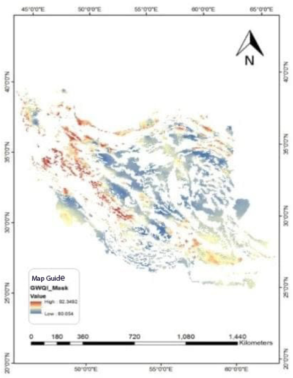
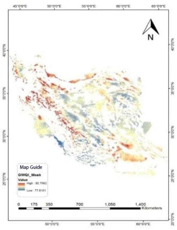
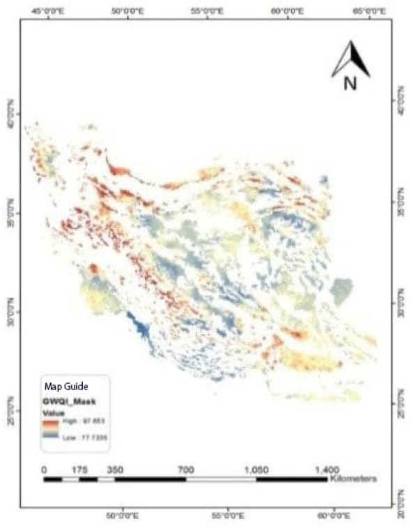
Figs. 10~12 indicate zoning with 25-year time intervals by the GWQI and the most optimal interpolation method for validation.
IV. Conclusions
In this study, the best zonings were initially chosen based on a comparison of standard errors utilizing geostatistical techniques and conclusive interpolation methods in order to do a full examination of the water quality condition in the country's aquifers. The continuous layers of Schuler, Wilcox, and GWQI indices were then computed based on the acquired raster maps. The results of this study are in line with the studies conducted by (Azizi and Mohammadzadeh, 2012), (Jamshidzadeh et al., 2011b), (Shabani, 2009), (Adhikary et al., 2011), (Hooshmand et al., 2011), and (Adhikary et al., 2011) for each parameter. In addition, this study is more consistent with the study conducted by (Delgado et al., 2010) in which a combination of geostatistical methods was introduced as an effective method for monitoring groundwater quality and the study performed by (Hooshmand et al., 2011), who indicated high accuracy of the Co-kriging method compared to Kriging method and also the studies conducted by (Soleimani et al., 2013), (Samin et al., 2012), (Gebrehiwot et al., 2011), all introducing Kriging method as a suitable method for preparing maps of groundwater quality parameters in terms of combination of approaches. Finally, it should be noted that in this study, we took a step higher than this research so that the results of each variable were presented based on a single parameter according to the most optimal description method, and a combination of these results was optimal was provided in general indicators and then in form of a better model of groundwater quality situation in Iran during 25 years. According to statistical summary table of Schuler index, calculated based on the zoned combined raster layers, in the plains of Iran, the non-drinkable class had a value of 1.36% during 12 years from 1995 to 2007, which was increased up to 1.54% during 2008-2020. In addition, the almost drinkable class showed a decrease from 15.15 to 13.65%; while the bad class in the country's plains accounted for 43.39% of the total area in the first 12-year period, but in the second 12-year period, this value was increased up to 48.40%. These changes were also reduced in the unsuitable and good classes and almost remained unchanged in the acceptable class. Therefore, according to the Schuler index, quality of drinking water has generally decreased in the country. Similarly, based on the statistical summary of the Wilcox index in the zoning of Iran, about 66.77% of the country’s plains were classified into the unsuitable class in the 12-year period from 1995 to 2020; this amount has increased to 70.59% during 2008-2020, attributing to the obvious decrease in water levels in the country's aquifers. At the same time, the value of average class has decreased from 25.34 to 21.97%; therefore, considering the changes in two classes of good and excellent, it can be concluded that the areas with high sensitivity have been severely eliminated in this period.
According to general investigation of the groundwater situation in Iran, as 70.59% of the aquifers have been considered as unsuitable for agricultural use, the crisis of groundwater quality becomes more apparent. This trend has intensified with the decrease in the groundwater level. Finally, for verifying the results extracted from the two mentioned indicators, using the GWQI, spatial changes in water quality were evaluated for 609 plains of the country. The results of long-term period indicated the values ranging between 77.73 - 97.65%. According to the general schema of the situation in the country’s groundwater resources as indicated in this study, it can be concluded that in addition to severe shortage of groundwater reserves in Iran, most of these resources are not considered desirable in terms of drinking and agricultural standards or at least they are considered at threshold of undesirable classes (IMOE, 1988). This indicates high sensitivity of Iranian aquifers to small changes in water level, which has been facing a more severe decline in recent years. Clearly, over-harvesting water in the agriultural sector could be the main reason for this finding. Therefore, it is recommended that required steps be taken to minimize water salinity by the assistance of state-of-the-art technologies and consequently increase the quality of groundwater for agricultural and drinking purposes. In this regard, serious efforts for implementing the plan to rehabilitate and balance the aquifers can be effective if it is actualized.
