1. 서  론

다공성 매질에서 비선형 흐름은 사력(rockfills), 자갈 하상(gravel beds) 그리고 폐기물 더미(waste dump)와 같은 매질 내 상대적으로 높은 침투유속에서 발생하며, 이러한 비선형 흐름에 대한 모델링은 지하수, 지반 그리고 환경공학과 같은 많은 분야에서 다루어지고 있다.

지난 십 수년 전부터 Darcy 법칙으로부터 관성력의 효과가 큰 다공성 매질을 통한 흐름으로 확장하기 위한 경험적 그리고 이론적 연구가 수행되어져 왔다(Skjetne and Auriault, 1999a,b). 일반적으로 다공성 매질에서 지하수 흐름을 해석하는데 적용되는 Darcy의 법칙(Darcy, 1856)은 다음과 같은 식으로 표현된다.

                               (1)

                            (2)

여기서 는 유속벡터 [m/sec], 는 투수계수 [m/sec], 는 수두 [m], 는 압력 [Pa], 는 밀도 [kg/m³], 는 중력가속도 [m/sec²] 그리고 는 위치수두 [m]이다.

Eqs. (1) and (2)로부터 Darcy 법칙은 다음과 같은 식으로 표현할 수 있다.

                       (3)

여기서 는 유체의 점성계수 [kg/(m·sec)] 그리고 는 다공성 매질의 고유 투수능 [m²]이다.

Helmig (1997)에 따르면 Bear and Bachmat (1986)은 Darcy 법칙을 유도할 때 관성과 시간 변화에 대한 효과를 무시하였다. 따라서 Darcy 법칙은 단지 매우 느린 흐름() 대해만 적용될 수 있으며, 여기서 레이놀즈 수()는 관성력과 점성력의 비로써 Eq. (4)와 같이 정의된다.

                                  (4)

여기서 는 동점성 계수 [m²/sec]이며, 은 다공성 매질의 특성길이(characteristic length)이다. 특성길이는 다공성 매질에 따라 달라지나 일반적으로 다공성 매질을 구성하는 입자의 지름으로 정의된다(Francher et al., 1933). Mayer et al. (2011)은 단위 체적당 다공성 매질을 구성하는 입자와 유체 사이의 접촉면적으로 정의되는 비접촉면적(specific interfacial area, =901 [1/m])을 이용하여 이 1/901 [m]로 산정하였다.

Skjetne (1995)는 다공성 매질에서 에 따라 유동 형태(flow regime)을 Fig. 1과 같이 5개로 분류하였다: 1=Darcy’s law, 2=Weak inertia, 3=Forchheimer (strong inertia), 4= Transition from Forchheimer to turbulence. 1은 관성력에 비해 점성력이 우세한 유동 형태이며, Darcy의 법칙이 적용될 수 있다. 2에 해당하는 weak inertia는 관성력이 점성력과 같은 정도가 됨을 의미하며, 그 이후에는 관성력이 지배적인 유동 형태에 해당된다.

Fig. 1

Flow regimes in a porous medium (Skjetne, 1995)

다공성 매질에서의 Darcy 법칙이 적용될 수 없는 즉 상대적으로 큰 유속, 즉 Fig. 1에서 유동 형태 3 이상인 유체흐름은 관성과 점성 그리고 압력 사이의 국부적인 비선형적 상호작용에 의해 특성지울 수 있다(Skjetne and Auriault, 1999a,b). 이러한 비선형적 효과는 Eq. (1)에 의해 예측된 압력손실보다 큰 압력손실을 발생시키며, 부가적인 비선형항의 도입될 필요가 있다. Forchheimer (1901)는 다공성 매질 내에서 유속이 증가함에 따라 점성효과보다는 관성효과가 흐름을 지배한다는 것을 설명하기 위해 Darcy 법칙에 유체의 운동에너지를 대표하는 관성항을 포함시킨 Eq. (5)를 제안하였다(Dullien, 1992).

                         (5)

여기서 와 는 상수이며, 다공성 매질의 공극율에 의존한다.

Muskat (1937), Green and Duwez (1951) 그리고 Cornell and Katz (1953)은 상수 와 를 유체와 다공성 매질을 구성하는 입자의 특성과 관계를 지었으며, Eq. (5)를 변형시켜 Forchheimer 식으로 알려진 Eq. (6)을 제시하였다.

                         (6)

여기서 는 Forchheimer 투수성 계수이며, 는 관성계수 또는 Forchheimer 계수이다. Eq. (6)에서 는 Eq. (3)에 있는 와 흐름 레짐의 차이(는 유동 형태 3이상 그리고 는 유동 형태 1에 해당)로 인해 동일하지 않다. 와 는 실험 또는 수치자료의 curve fitting을 통해 결정되는 상수이다.

Forchheimer 식은 Muskat (1937), Ahmed and Sunuda (1969), Scheidegger (1960), Chauveteau and Thirriot (1967), Wright (1968), Greertsma (1974), Firoozabadi and Katz (1979) 그리고 Tiss and Evans (1989)에 의한 실험을 통해 관성력이 지배적인 흐름에 적용될 수 있음이 증명되었다.

Eq. (6)을 변형하여 마찰계수 와 수정 레이놀즈 수 와의 관계식으로 표현하면 다음과 같다(Churchill, 1988).

                                (7)

여기서 그리고 이다.

Mayer et al. (2011)은 에 대해 Eq. (8)과 같은 경험식을 제안하였다.

                               (8)

여기서 는 비접촉면적으로 Eq. (4)에 나와 있는 특성길이의 역수이다. 본 연구에서는 마찰계수와 레이놀즈 수의 관계를 분석하는데 있어 Eq. (8)과 Eq. (4)를 적용하였다.

최근 Cheng et al. (2008)은 다공성 매질을 통한 비선형 흐름에 대한 이차 법칙(quadratic law)과 멱 법칙(power law)의 적용성을 검토하기 위해 물리적 실험과 수치적 실험을 수행하였으며, 이차 법칙은 선형과 비선형 흐름 둘 다에 대해 적용이 가능하나 멱 법칙을 적용하는 것은 타당하지 않다는 결론을 제시하였다. Skjetne (1995)는 비압밀 그리고 압밀 다공성 매질 및 균열 시스템에 대해 Forchheimer 식의 적용 타당성을 조사하기 위한 연구를 수행하였으며, 다양한 유속 조건에 대해 Forchheimer 식이 적용 가능하다는 것을 제안하였다. 그러나 다공성 매질 내에 유체 흐름에 영향을 미치는 유체의 점성계수, 매질의 투수성 계수 그리고 공극율과 같은 물리적 특성의 변화에 따른 압력 변화 및 마찰계수와 와의 관계 변화 등에 대한 연구는 국내외적으로 거의 없는 실정이다.

본 연구에서는 3차원 상용 유동 모의 및 분석 모형인 ANSYS CFX (Jeong, 2014; 2015)를 이용하여 다공성 매질의 물리적 특성 변화에 따른 압력과 유속의 변화 관계, 와의 관계 그리고 Eq. (6)에 제시된 계수 등을 수치적 방법을 통해 조사 및 분석을 수행하였다.

2. 적용된 수치모형의 검증

본 연구에서 적용된 수치모형의 검증을 위해 Mayer et al. (2011)이 균일하게 배열된 벌집(honeycomb) 형태(Fig. 2(b)의 공간들이 내재되어 있는 다공성 실린더형 구조체(Fig. 2(a))를 대상으로 양 끝단 압력경사의 변화에 따른 비선형적 유동특성을 분석하기 위해 수행한 실내 실험결과를 이용하였다.

Fig. 2

Photograph of experimental set-up (a) and Porous structure used in experiments

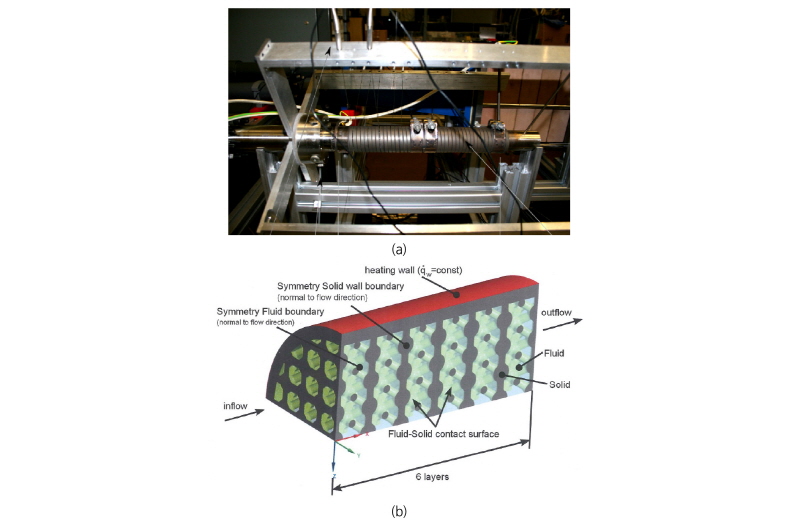
실험에서 사용된 다공성 실린더형 구조체의 길이는 0.295 m 그리고 직경은 0.03 m이며, 구조체 내부를 통과하는 유체는 등온상태(isothermal state)의 공기로 가정하였다. Table 1은 실험에 적용된 공기의 물리적 특성(밀도와 점성계수)과 실험을 통해 분석된 압력경사의 변화에 따른 유속과 레이놀즈수를 나타낸 것이다.

Table 1. Physical property of air and experimental results

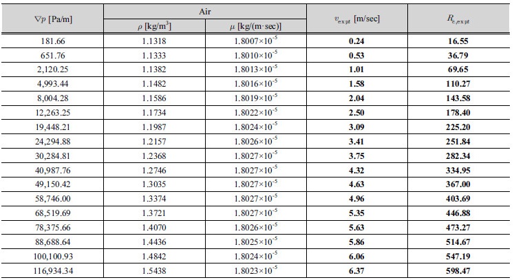
검증을 위한 수치모의에서 적용된 다공성 구조체는 실험에서 수행한 것과 동일하나 Fig. 3(a)에서처럼 일방향 흐름(unidirectional flow)이고 대칭 형태이기 때문에 전체 구조체의 4분의 1만 고려하였다. 본 모의에서 흐름은 양 끝단의 압력차에 의해 지배되며, 양 끝단에는 Dirichlet 경계조건을 적용하였다. 유입경계에서의 압력은 Table 1의 압력경사를 이용하여 계산하였으며, 유출경계에는 대기압 조건(100,000 Pa)을 적용하였다. 구조체의 벽면은 no flow 즉 Neumann 경계조건을 적용하였으며, 내부 측벽과 바닥벽에는 symmetry 경계조건을 적용하였다.

Fig. 3(b)는 육면체 요소(hexahedral element)들로 구축된 구조적 격자망을 나타낸 것으로 절점은 496,184개 그리고 셀은 478,525개로 구성되었다. 다공성 구조체의 고유투수계수(intrinsic permeability, )는 실험을 통해 산정된 5.73×10^-8 m² 그리고 공극율(porosity, )은 0.558을 적용하였다.

Fig.3

Model domain with boundary conditions (a) and uniform mesh with hexahedral elements (b)

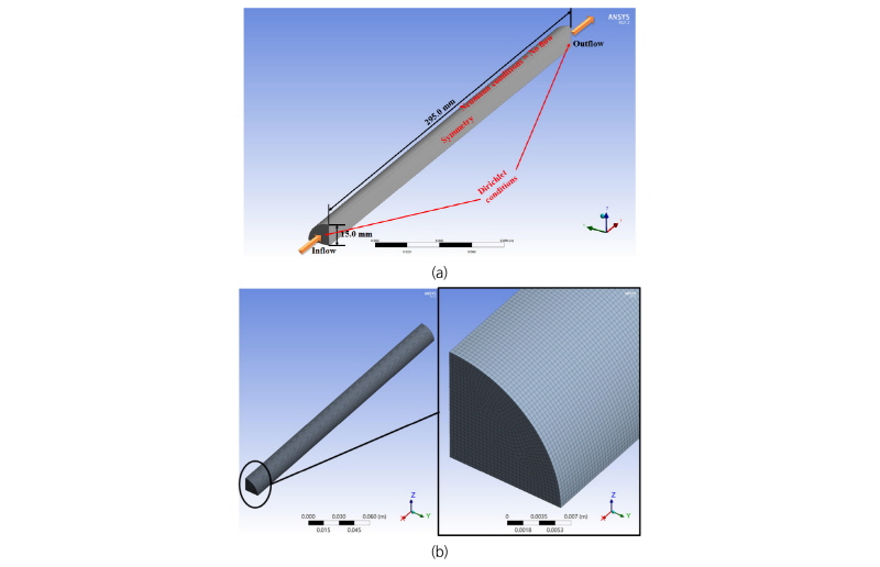
Fig. 4는 적용된 17개의 압력경사() 중에서 세 가지 경우 즉 가 181,660와 24,294.88 그리고 116,934.34 Pa/m에 대한 압력분포를 나타낸 것으로 계산된 압력은 다공성 구조체를 따라 유입경계에서부터 유출경계까지 선형으로 변화되는 것을 볼 수 있다.

Fig.4

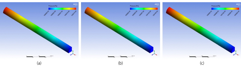
Pressure distribution across porous structure: (a) = 181.660 Pa/m (b), = 24,294.88 Pa/m and (c) = 116,934.34 Pa/m

Fig. 5는 압력분포의 경우와 마찬가지로 세 가지 에 대한 유속분포를 나타낸 것으로 계산된 유속은 다공성 구조체를 따라 유입경계에서부터 유출경계까지 일정한 값을 유지하고 있는 것을 볼 수 있다.

Fig.5

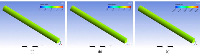
Velocity distribution across porous structure: (a) = 181.660 Pa/m (b), = 24,294.88 Pa/m and (c) = 116,934.34 Pa/m

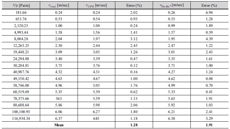
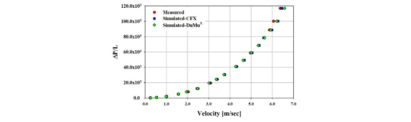
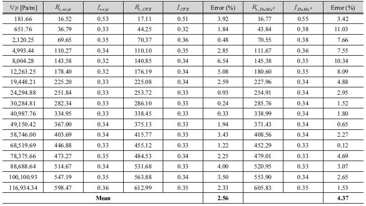
Table 2는 실험을 통해 산정된 유속과 수치모형에 의한 유속을 비교한 것이다. 본 연구에서 적용된 수치모형 이외에 Jambhekar (2011)가 DuMu^X 모형을 이용하여 동일한 조건 하에서 모의한 유속을 비교하였다. DuMu^X 모형은 다공성 매질에서 유체흐름과 용질 이송 과정을 모의하기 위해 독일 Stuttgart 대학에서 개발한 오픈 소스 소프트웨어이다. 유속과 마찰계수에 대한 오차분석에 적용된 식은 다음과 같다.

Table 2. Comparison of experimental and numerical velocities

                 (9)

비교결과 본 연구에서 적용된 수치모형으로부터의 유속은 실험을 통한 유속과 각각의 압력경사에 대해 비교적 잘 일치하는 것으로 나타났으며, 평균오차는 1.28%로 산정되었다. DuMu^X 모형으로부터의 유속의 평균오차는 1.91%로 본 연구에서 적용된 수치모형이 0.63% 보다 정확한 것으로 산정되었으나 DuMu^X 모형 적용 시 격자망의 조밀도가 상대적으로 낮기 때문에(셀의 개수가 2배 정도 작음) 실제적으로는 거의 차이가 없는 것으로 판단된다. Fig. 6은 Table 2의 비교결과를 그래프로 나타낸 것이다.

Fig.6

Comparison between measured and simulated velocity distribution

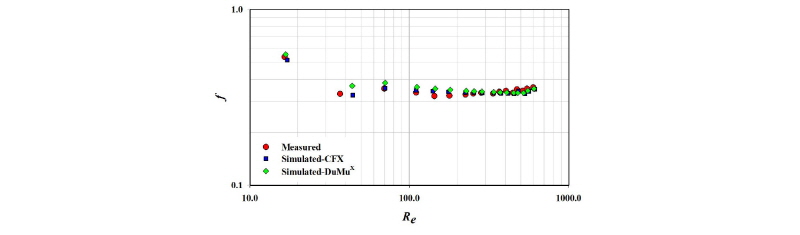
비교결과 본 연구에서 적용된 수치모형으로부터 계산된 결과는 실험을 통해 산정된 결과와 비교적 잘 일치하는 것으로 나타났으며, 평균오차는 2.56%로 산정되었다. DuMu^X 모형으로부터의 평균오차는 4.37%로 본 연구에서 적용된 수치모형이 1.72% 보다 정확한 것으로 산정되었으나 DuMu^X 모형 적용 시 격자망의 조밀도가 상대적으로 낮기 때문에(셀의 개수가 2배 정도 작음) 실제적으로는 거의 차이가 없는 것으로 판단된다. Fig. 7은 Table 3의 비교결과를 그래프로 나타낸 것이다.

Fig.7

Comparison between measured and simulated friction coefficient

Table 3. Comparison of experimental and numerical friction coefficient,

3. 다공성 매질의 물리적 특성 변화에 따른 유체흐름 모의 및 결과 분석

3.1 공극율()의 변화

본 모의에서는 다공성 매질의 공극율 변화( = 0.3, 0.4 그리고 0.5)에 대해 압력경사()에 따른 유속() 및 마찰계수()의 변화를 분석하였다. 투수능(와 동점성 계수()는 각각 1.0×10^-8 m²과 1.0×10^-7 m²/sec로 의 변화에 대해 동일하게 적용하였다.

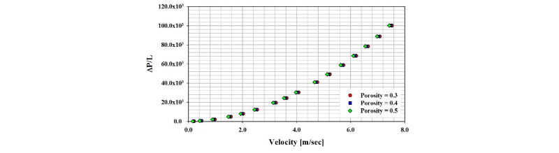
Fig. 8은 의 변화에 따른 와 의 관계를 나타낸 것으로 의 증가에 따라 이 비선형으로 증가하는 것으로 나타났으며, 이러한 경향은 Cheng et al. (2008)과 Jambhekar (2011)의 실험적 연구에서 제시된 경향과 거의 동일하다. Table 4는 네 개의 대표적인 에서의 의 변화에 따른 을 비교한 것이며, 괄호 내의 값은 Eq. (4)를 통해 계산된 레이놀즈 수()를 나타낸 것이다. 이 181.66 Pa/m인 경우 가 0.3일 때의 에 비해 0.4에서는 0.86배 그리고 0.5에서는 0.76배 작게 산정되었다. 그러나 그 이후에서는 이러한 차이가 감소되며, 이 116,934.34 Pa/m인 경우 이 0.3일 때의 에 비해 가 0.4와 0.5의 경우 각각 0.99배와 0.99배 작게 산정되어 거의 차이가 없음을 알 수 있다.

Fig.8

Comparison of relationship with porosity

Table 4. Comparison of velocities at four values of with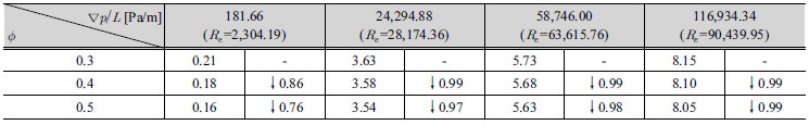

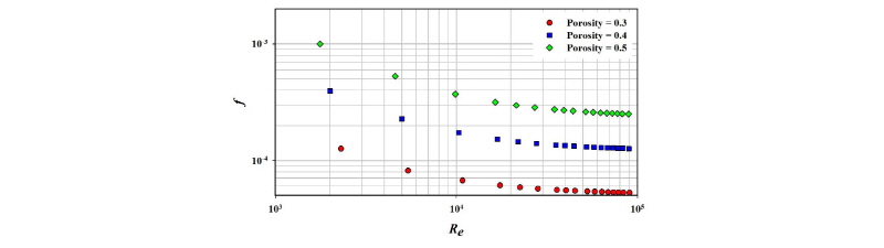
Fig. 9는 의 변화에 따른 -의 관계를 나타낸 것으로 의 증가에 따라 의 값이 감소하는 경향을 나타냈었다. 값 모두에서 의 값이 약 22,000 보다 작은 구간에서는 급격히 감소하나 그 이후부터는 매우 느리게 감소하면서 일정한 값에 점근하는 결과를 나타내었다. Table 5는 네 개의 대표적인 에서 의 변화에 따른 의 변화를 비교한 것이다. 이 181.66 Pa/m인 경우 가 0.3일 때의 에 비해 0.4에서는 3.13배 그리고 0.5에서는 7.91배 크게 산정되었다. 그러나 그 이후에서는 이러한 차이가 감소되며, 이 24,294.88 Pa/m인 경우 이 0.3일 때의 에 비해 가 0.4와 0.5의 경우 각각 2.46배와 5.00배로 작게 산정되었다. 또한 이 116,934. Pa/m인 경우 가 0.3일 때의 에 비해 가 0.4와 0.5의 경우 각각 2.40배와 4.74배로 크게 산정되었으며, 이 24,294.88 Pa/m인 경우와 거의 비슷한 결과를 보였으며, 일정한 값에 점근하는 경향을 나타내었다.

Fig.9

Comparison of relationships with porosity

Table 5. Comparison of friction coefficients at four values of with

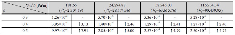
3.2 동점성 계수()의 변화

본 모의에서는 다공성 매질 내 유체 동점성 계수의 변화( = 1.0×10^-5, 1.0×10^-6 그리고 1.0×10^-7 m²/sec)에 대해 에 따른 및 의 변화를 분석하였다. 다공성 매질의 와 는 각각 0.5와 1.0×10^-8 m²로 의 변화에 대해 동일하게 적용하였다.

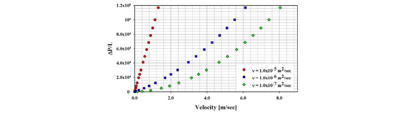
Fig. 10은 의 변화에 따른 -의 관계를 나타낸 것으로 가 1.0×10^-5 m²/sec의 경우 의 증가에 따라 이 선형으로 증가하는 것으로 나타났으나 가 1.0×10^-6 그리고 1.0×10^-7 m²/sec의 경우에는 다소 비선형으로 증가하는 것으로 나타났다. Table 6은 네 개의 대표적인 에서 의 변화에 따른 을 비교한 것이다. 이 181.66 Pa/m인 경우 가 1.0×10^-5 m²/sec일 때의 에 비해 1.0×10^-6 m²/sec에서는 10.50배 그리고 1.0×10^-7 m²/sec에서는 79.50배 크게 산정되었다. 그러나 그 이후에서는 이러한 차이가 급격하게 감소되며, 이 116,934.34 Pa/m인 경우 이 1.0×10^-5 m²/sec일 때의 에 비해 가 1.0×10^-6와 1.0×10^-7 m²/sec의 경우 각각 4.68배와 6.16배로 크게 산정되었다.

Fig. 10

Comparison of relationship with kinematic viscosity

Table 6. Comparison of velocities at four values of with

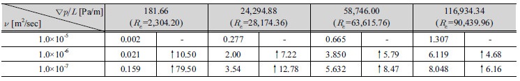
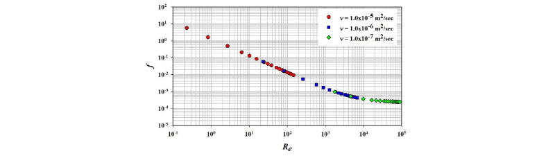
Fig. 11은 의 변화에 따른 -의 관계를 나타낸 것으로 의 증가에 따라 의 값이 감소하는 경향을 나타냈었다. 의 값이 1.0×10^-5 m²/sec의 경우 가 2,120.25 Pa/m까지 의 값이 급격하게 감소하다가 그 이후부터 일정한 값에 수렴하면서 매우 느리게 감소한다. 이러한 경향은 의 값이 1.0×10^-6 과 1.0×10^-7 m²/sec 경우에 대해서도 동일한 경향을 나타내었다. Table 7은 네 개의 대표적인 에서 에 따른 의 변화를 비교한 것이다. 이 181.66 Pa/m인 경우 가 1.0×10^-5 m²/sec일 때의 에 비해 가 1.0×10^-6 m²/sec에서는 99.22배 그리고 1.0×10^-7 m²/sec에서는 5,814.60배 작게 산정되었다. 그러나 그 이후에서는 이러한 차이가 급격하게 감소되며, 이 24,294.88 Pa/m인 경우 가 1.0×10^-5 m²/sec일 때의 에 비해 가 1.0×10^-6와 1.0×10^-7 m²/sec의 경우 각각 69.23배와 300.00배로 작게 산정되었다. 또한 이 116,934. Pa/m인 경우에는 각각 23.75배와 47.50배로 작게 산정되었다.

Fig. 11

Comparison of relationships with kinematic viscosity

Table 7. Comparison of friction coefficients at four values of with

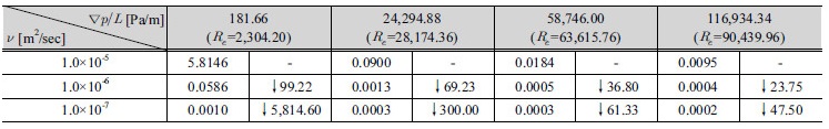
3.3 투수능()의 변화

본 모의에서는 다공성 매질 내 유체의 투수능의 변화( = 1.0×10^-8, 1.0×10^-9 그리고 1.0×10^-10 m²)에 대해 적용된 에 따른 및 의 변화를 분석하였다. 다공성 매질의 와 는 각각 0.5와 1.0×10^-7 m²/sec로 의 변화에 대해 동일하게 적용하였다.

Fig. 12는 의 변화에 따른 -의 관계를 나타낸 것으로 가 1.0×10^-8 m²의 경우 의 증가에 따라 유속이 거의 선형으로 증가하는 것으로 나타났으나 가 1.0×10^-9 그리고 1.0×10^-10 m²과 같이 감소함에 따라 비선형으로 증가하는 경향을 나타내었다. Table 8은 네 개의 대표적인 에서 의 변화에 따른 유속을 비교한 것이다. 이 181.66 Pa/m인 경우 가 1.0×10^-8 m²일 때의 유속에 비해 1.0×10^-9 m²에서는 6.96배 그리고 1.0×10^-10 m²에서는 60.33배 크게 산정되었다. 그러나 그 이후에서는 이러한 차이가 급격하게 감소되며, 이 116,934.34 Pa/m인 경우 가 1.0×10^-8 m²일 때의 유속에 비해 가 1.0×10^-9와 1.0×10^-10 m²의 경우 각각 1.25배와 5.02배로 산정되었다.

Fig. 12

Comparison of relationship with intrinsic permeability

Table 8. Comparison of velocities at four values of with

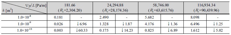
Fig. 13은 의 변화에 따른 -의 관계를 나타낸 것으로 앞 절의 두 물리량 경우와 마찬가지로 의 증가에 따라 의 값이 감소하는 경향을 나타냈었다. 의 값이 1.0×10^-8 m²의 경우 가 2,120.25 Pa/m까지 의 값이 급격하게 감소하다가 그 이후부터 일정한 값에 수렴하면서 매우 느리게 감소한다. 이러한 경향은 의 값이 1.0×10^-6 과 1.0×10^-7 m²/sec 경우에 대해서도 동일한 경향을 나타내었다. Table 9는 네 개의 대표적인 에 대해 에 따른 의 변화를 비교한 것이다. 이 181.66 Pa/m인 경우 가 1.0×10^-8 m²일 때의 에 비해 가 1.0×10^-9 m²에서는 48.25배 그리고 1.0×10^-10 m²에서는 4,743.75배 작게 산정되었다. 그러나 그 이후에서는 이러한 차이가 급격하게 감소되며, 이 24,294.88 [Pa/m]인 경우 가 1.0×10^-8 m²일 때의 에 비해 가 1.0×10^-9와 1.0×10^-10 m²의 경우 각각 2.00배와 61.00배로 크게 산정되었다. 또한 이 116,934. Pa/m인 경우에는 각각 2.00배와 32.00배로 크게 산정되었다.

Fig. 13

Comparison of relationships with intrinsic permeability

Table 9. Comparison of friction coefficients at four values of with

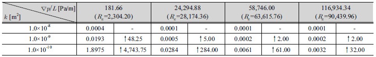
4. 결  론

본 연구에서는 다공성 매질의 공극율, 유체의 동점성 계수 그리고 투수능과 같은 물리적 특성의 변화에 따른 유체 흐름의 비선형 거동에 대한 수치적 분석을 수행하였으며, 다음과 같은 결론을 얻었다.

1. 본 연구에서 적용된 수치모형의 검증을 위해 Mayer et al. (2011)이 수행한 실험 자료를 이용하였으며, 검증 결과 압력경사와 유속과의 관계 그리고 마찰계수와 레이놀즈 수와의 관계에 있어 실험결과와 비교적 잘 일치하는 결과를 얻었으며, Jambhekar (2011)에 의해 수행된 DuMu^X 모형을 통한 모의 결과와도 비교적 잘 일치하였다.

2. 다공성 매질에서 유체흐름의 비선형 거동에 가장 큰 영향을 미치는 물리적 특성은 유체의 동점성 계수가 됨을 알 수 있었다. 압력경사가 181.66 Pa/m에서 동점성 계수가 1.0×10^-5 m²/sec일 때 산정된 유속을 기준으로 할 때 1.0×10^-6 m²/sec에서는 10.50배 그리고 1.0×10^-7 m²/sec에서는 79.50배 크게 산정되었다. 마찰계수의 경우 동점성 계수가 1.0×10^-5 m²/sec일 때 산정된 마찰계수를 기준으로 할 때 1.0×10^-6 m²/sec에서는 99.22배 그리고 1.0×10^-7 m²/sec에서는 5,814.60배 작게 산정되었다.

3. 동점성 계수는 클수록 압력경사의 증가에 따라 유속은 선형으로 증가되는 경향을 나타내었으나 투수능의 경우에는 작을수록 선형으로 증가되는 경향을 나타내었다. 이는 동점성 계수가 클수록 관성력보다는 점성력이 상대적으로 우세하며, 투수능은 작을수록 관성력보다는 점성력이 상대적으로 우세하다는 것을 의미하는 것으로 판단된다.