

1. 서 론
2. 자료 및 방법
2.1 가설(Hypothesis)
2.2 자료수집
2.3 연구방법
3. 결과 및 고찰
3.1 기존 연구결과를 활용한 인공지능 모델 예측결과 분석
3.2 허용가능한 오차범위 추정
4. 결 론
1. 서 론
지하수는 지표수와 함께 농업, 공업 및 생활용수로 사용가능한 중요한 수자원이다. 특히 섬 지역의 경우 지하수의 의존율이 지표수보다 높으며, 제주도의 경우 전체 용수의 81%가 지하수에 해당하여(JSSGP, 2018) 높은 용수비율을 차지하고 있으므로 지하수의 지속가능한 이용을 위해 지하수의 관리는 매우 중요하다. 또한 지하수의 수량적인 관점에 있어서 안정적인 지하수의 이용을 위해 기상변화 및 인간의 인위적 활동에 의한 지하수위의 변동성에 대한 연구가 반드시 필요하다.
지하수위를 예측하고 변동성을 분석하기 위해 지하수 수치모델인 MODFLOW (McDonald and Harbaugh, 1988)가 널리 사용되고 있으며(Mohanty et al., 2013), 완전 결합형 분포형 수치모델인 HydroGeosphere (Therrien, 1992; Brunner and Simmons, 2012) 등도 사용되고 있다(Ala-Aho et al., 2015). 지하수 수치모델은 유한차분법, 유한요소법 또는 두 방법을 조합한 연산방법과 Darcy 법칙과 질량보존 법칙 등 물리적 법칙 그리고 공간적으로 다른 투수계수 및 수치표고모델(Digital Elevation Model)등을 포함한 다양한 물리적 자료를 사용하여 지하수의 흐름을 모의하고 대상지점의 지하수위를 계산한다(Todd and Larry, 2004). 따라서 지하수 수치모델들을 사용하여 비균질한 지하수 시스템을 모의하기 위해서는 다양한 시공간적 자료가 필요하며(Barthel and Banzhaf, 2016) 많은 비용과 긴 모의시간이 필요하다(Maxwell et al., 2015). 지하수 수치모델은 복잡한 수문학적 프로세스의 단순화(White et al., 2014) 및 모의 격자의 크기(discretization) 설정에 따른 불확실성(White et al., 2020), 그리고 양질의 자료 취득의 어려움으로 인해 지하수위를 적절히 모의하는데 어려움이 있다(Sun et al., 2016). 이에 대한 대안적인 방법으로 다양한 자료의 상관관계를 이용하여 지하수위를 예측하는 인공지능 모델을 활용할 수 있다. 데이터기반 모델인 인공지능 모델은 목표(반응)변수(지하수위 등)와 목표 변수에 관련된 설명변수(강수 및 취수량 등) 간의 관련정도(연결강도)를 복수의 은닉층 내의 셀들로 구성된 망을 사용하여 학습함으로써 지하수위를 산정한다. 따라서 인공지능 모델은 지하수 수치모델에 필요한 양질의 다양한 공간적 자료의 수집 및 이용의 부담이 없다. 이러한 인공지능 모델의 장점을 바탕으로, 지난 20년 동안 인공지능 모델을 활용한 다양한 연구가 성공적으로 수행되었다(Rajaee et al., 2019). 최근에는 Long Short-Term Memory (LSTM) network 등 딥러닝 인공지능 모델을 사용하여 지하수위를 예측하는 연구가 증가하고 있다(Jeong and Park, 2019; Shin et al., 2020).
과거 20년 동안 전 세계 다양한 지역에 대해 인공지능 모델을 활용하여 지하수위를 예측한 연구들을 살펴보면, 적절히 모의된 지하수위 예측결과들은 연구별로 서로 다른 평균제곱근오차(root mean square error, RMSE) 등 상이한 예측오차들을 보였다(Coulibaly et al., 2001; Daliakopoulos et al., 2005; Mirzavand et al., 2015; Zhang et al., 2018; Afzaal et al., 2020). 따라서 인공지능 모델을 활용하여 지하수위를 예측한 경우 그 결과의 적절성을 판단하는데 어려움이 있을 수 있다. 하지만 조사결과 지하수위 예측결과의 적절성 판단을 위한 평가기준을 제시한 연구는 충분하지 않았다. 유사한 연구로써 Moriasi et al. (2007)은 수문모델의 지표수 유출모의에 대해 모의결과의 적절성을 판단하기 위한 지표를 제시하였으나 지하수위 예측에 대한 적절성 기준은 제시하지 않았다. 앞에서 언급한 5편의 인공지능 모델 활용 지하수위 예측연구들은 서로 다른 예측오차 뿐만 아니라 서로 다른 관측지하수위 변동폭을 보였다. 제주도와 같은 섬 지역의 경우 해안 지역의 얕은 대수층부터 중산간 지역의 깊은 대수층까지 지역마다 다양한 깊이의 대수층과 관측지하수위 변동폭을 보이고 있기 때문에(JSSGP, 2018) 연구대상 지역마다 서로 다른 지하수위 예측오차를 보일 수 있다. 또한 관측지하수위의 변동폭이 크고 변동형상이 복잡할수록 인공지능 모델을 활용한 지하수위 예측이 어려워져 예측오차가 증가할 수 있다. 이러한 경우 적절한 평가기준 없이는 인공지능 모델의 지하수위 예측결과에 대한 적절성을 객관적으로 판단하기 어려울 수 있다. 또한 큰 첨두유량과 짧은 감수곡선시간을 보이는 지표수 수문곡선은 상대적으로 작은 첨두지하수위와 상대적으로 긴 감수지하수위시간을 보이는 지하수위 시계열자료와 변동특성이 다르기 때문에 지표수 수문모델 유출모의에 대한 평가기준(Moriasi et al., 2007)을 인공지능 모델의 지하수위 예측평가에 적용하는 것은 적절하지 않을 수 있다. 따라서 인공지능 모델에 의한 지하수위 예측결과의 평가기준에 대한 연구가 필요하다.
본 연구의 목적은 인공지능 모델을 활용하여 지하수위를 예측한 경우 예측결과에 대한 오차가 어느 정도 이상이면 허용가능한지에 대한 기준을 마련하는데 있다. 객관적으로 타당한 허용가능한 예측오차 범위를 설정하기 위해 전 세계를 대상으로 수행한 가능한 모든 관련 연구들을 수집하였다. 또한 허용가능한 최소의 기준을 마련하는 것이 목적이므로 기존 연구들에서 적절하다고 제시된 연구결과들 중 가장 낮은(나쁜) 결과들을 추출하여 분석하였다. 본 연구에서 사용한 연구방법은 2절에 상세히 기술하였으며 결과 및 결론은 각각 3절과 4절에 제시하였다.
2. 자료 및 방법
2.1 가설(Hypothesis)
1절에서 기술하였듯이, 연구대상지역 관측지하수위의 변동폭이 크고 변동횟수가 많아 지하수위의 변동형태가 복잡할수록 인공지능 모델을 활용한 지하수위 예측은 어려워질 수 있으며 이에 따라 예측오차는 증가할 수 있다. 따라서 본 연구에서는 다음과 같은 가설을 설정하였다.
가설: “관측지하수위의 최대변동폭이 클수록 지하수위 예측오차는 증가한다.”
인공지능 모델은 학습(training)기간의 자료를 통해 얻은 정보(추정된 매개변수값)를 사용하여 검증(validation) 또는 테스트(testing) 기간의 지하수위를 예측한다. 즉, 검증 또는 테스트 기간의 예측결과(예측오차)는 학습기간의 정보와 분리될 수 없다. 따라서 본 연구에서 사용한 관측지하수위의 최대변동폭은 학습기간을 포함한 전체 관측지하수위의 최대변동폭이다. 예를 들어, 한 개의 특정 관정 관측지하수위의 최대변동폭은 이 한 개 관정의 전체 관측지하수위 시계열 자료 중 최대값과 최소값의 차이다.
2.2 자료수집
전 세계 다양한 지역의 지하수위 예측결과를 종합적으로 분석하기 위해 다양한 국제저널들에 게재된 논문들을 수집하였다. 인공지능 모델을 활용한 최근까지의 가능한 모든 지하수위 예측 연구들을 사용하기 위해 2001년부터 2020년까지 20년간 발간된 논문들을 수집하였으며 그 중 본 연구의 목적과 부합된 논문들을 선정하였다. 논문의 선정기준은 다음과 같다.
∙영향력지수(impact factor)를 가진 국제적으로 검증된 저널에 게재된 논문이어야 한다.
∙연구방법 및 결과가 타당해야 한다.
∙모의결과에 대한 RMSE와 전체 관측 및 모의 지하수위 곡선들이 제시되어 있어야 한다.
∙가능하면 Nash‒Sutcliffe efficiency (NSE) (Nash and Sutcliffe, 1970), 결정계수(R2) 또는 상관계수 등 모의결과 적절성 평가를 위한 통계지수가 포함되어 있어야 한다.
그 결과 총 35편의 인공지능 모델을 활용한 지하수위 예측 논문들을 선정하였으며 이 논문들에서 제시된 연구결과들을 본 연구의 분석에 사용하였다.
2.3 연구방법
본 연구의 목적은 1절에서 기술하였듯이 인공지능 모델을 활용하여 모의된 지하수위 예측결과의 적절성을 평가하기 위한 최소의 기준을 설정하는 것이다. 따라서 선정한 35편의 논문들에 대해 아래와 같은 방법으로 본 연구에 필요한 자료들을 추출하였다.
1)각 논문별로 연구에 사용된 복수의 인공지능 모델들 중 가장 좋은 예측결과들을 도출한 최적 인공지능 모델을 선택한다.
2)허용가능한 최대 지하수위 예측오차를 추정하는 것이 목적이므로, 선택한 최적 인공지능 모델에 의한 예측결과들 중 RMSE, NSE, R2 또는 상관계수가 가장 낮은(나쁜) 모의결과를 선택한다. 예를 들어, 연구대상 지역이 3개 지역이라면 그 중 가장 나쁜 모의결과가 나온 지역의 결과를 선택한다.
3)선택한 가장 나쁜 모의결과에 대해 RMSE, NSE, R2 또는 상관계수를 추출한다. 또한 관측지하수위의 최대변동폭(m) 및 검증 또는 테스트기간에 대한 최대오차(m)를 추출한다.
그리고 이 추출한 자료들을 사용하여 지하수위 변동특성을 분석하였다. 또한 추출된 자료들을 사용하여 선형회귀분석을 수행하였으며, 선형회귀분석과 추출된 적절성 평가지수의 통계분석을 통해 인공지능 모델에 의한 지하수위 예측오차가 어느정도까지 허용 가능한지 판단할 수 있는 허용가능한 오차범위를 제시하였다. 유의사항으로서, 선형회귀분석을 통해 2.1절에서 제시한 가설을 검증하였으며, 유의확률을 이용한 귀무가설 검증방법은 사용하지 않았다.
3. 결과 및 고찰
3.1 기존 연구결과를 활용한 인공지능 모델 예측결과 분석
본 연구와 관련하여 선정된 35편의 논문들을 분석한 결과는 Table 1과 같다. Table 1의 결과에서 볼 수 있듯이 이 연구들은 2001년부터 2020년까지 한국, 중국, 인도, 그리스 및 미국 등을 포함한 전 세계 다양한 지역을 대상으로 수행하였다. 사용된 최적 인공지능 모델은 Artificial Neural Network (ANN), Support Vector Machine (SVM) 및 LSTM 등 총 13개의 다양한 모델들이며, 모의 시간단위는 시, 일, 주 및 월 단위로써 다양한 모의시간단위를 사용하였다. 따라서 이 연구들은 인공지능 모델을 활용한 검증된 대표적인 결과들이라고 할 수 있다.
분석결과, 이 연구들의 관측지하수위 최대변동폭은 0.45 ~ 72 m의 넓은 범위를 보였으며 이것은 대상 지역들의 지하수위가 다양한 변동특성을 보인다는 것을 의미한다(Table 1(c)). 검증 또는 예측기간의 허용가능한 가장 낮은(나쁜) 모의결과에 대한 RMSE는 0.052 ~ 3.6 m의 범위(Table 1(d))를 보였으며 최대오차는 0.1 ~ 14 m로써 상대적으로 큰 범위를 나타내었다(Table 1(f)). 이것은 예상하였듯이 관측지하수위의 변동성이 클수록 모의지하수위의 오차는 증가한다는 것을 의미한다.
관측지하수위 최대변동폭 대비 모의지하수위 RMSE의 비율은 2.4 ~ 27.1%의 범위를 보였으며 평균값은 9.6%를 나타내었다(Table 1(e)). 그리고 관측지하수위 최대변동폭 대비 모의지하수위 최대오차의 비율은 7.7 ~ 48.0%의 범위를 보였으며 평균값은 24.0%를 나타내었다(Table 1(g)). 따라서 최대오차 비율의 평균값(24.0%)는 RMSE 비율의 평균값(9.6%) 보다 두 배 이상 컸다. 이것은 검증 또는 예측기간에 대한 RMSE는 오차들의 평균으로 인해 비록 상대적으로 작을 수 있지만 1개의 특정 예측일자(time step)의 오차는 매우 클 수 있다는 것을 의미한다. 만약 인공지능 모델을 활용하여 익월의 평균지하수위를 예측하는 경우 1개 예측 월의 지하수위값은 관측 지하수위값과 매우 큰 차이를 보일 수 있다. 따라서 특정 기간에 대한 허용가능한 오차범위의 추정 뿐만 아니라 1개의 특정 일(time step)에 대한 허용가능한 오차범위의 추정 또한 중요하다. 이 허용가능한 오차범위의 추정은 3.2절에 기술하였다.
Table 1.
Analysis of existing research results related to groundwater level prediction using artificial intelligence (AI) models
| No. |
Authors (year) | Study area |
Best AI model |
Time step |
(a) NSE of valida- tion or testing period |
(b) R2 of valida- tion or testing period |
(c) Maximum fluctuation width of observed groundwater level (m) |
(d) Allowable worst RMSE of validation or testing period (m) |
(e) Ratio of RMSE (%) ((d)/(c) ×100) |
(f) Allowable worst max- imum error of validation or testing period (m) |
(g) Ratio of maxi- mum error (%) ((f)/(c) ×100) |
| 1 | Coulibaly et al. (2001) |
Gondo aquifer, Burkina Faso (West Africa) | RNN | Monthly | - | - | 6.5 | 0.390 | 6.0 | 0.5 | 7.7 |
| 2 | Daliakopoulos et al. (2005) |
Island of Crete, Greece | ANN | Monthly | - | 0.985 | 44.5 | 2.110 | 4.7 | 4 | 9.0 |
| 3 | Nayak et al. (2006) |
Central Godavari Delta System, India | ANN | Monthly | - | - | 2.3 | 0.589 | 25.6 | 1 | 43.5 |
| 4 | Krishna et al. (2008) |
Andhra Pradesh state, India | ANN | Monthly | 0.7549 | 0.774 | 2.8 | 0.210 | 7.5 | 0.4 | 14.3 |
| 5 | Yang et al. (2009) |
Western Jilin, China | ANN | Monthly | 0.79 | - | 3 | 0.090 | 3.0 | 0.25 | 8.3 |
| 6 | Chen et al. (2010) |
Southern Taiwan | RBN | Monthly | 0.592 | - | 12 | 0.789 | 6.6 | 1.1 | 9.2 |
| 7 | Adamowski and Chan (2011) |
Quebec, Canada |
Wavelet- ANN | Monthly | 0.869 | 0.884 | 4.5 | 0.553 | 12.3 | 1.2 | 26.7 |
| 8 | Chen et al. (2011) |
Southern Taiwan | ANN | Monthly | 0.887 | - | 3.3 | 0.363 | 11.0 | 0.7 | 21.2 |
| 9 | Yoon et al. (2011) |
Beach of the Donghae city, South Korea | SVM |
Six- hourly | - | - | 2 | 0.154 | 7.7 | 0.5 | 25.0 |
| 10 | Kisi and Shiri (2012) |
Illinois State, USA |
Wavelet- ANFIS | Daily | - | 0.984 | 22 | 0.795 | 3.6 | 7 | 31.8 |
| 11 | Rakhshandehroo et al. (2012) |
Shiraz plain, Iran | ANN | Monthly | - | 0.883 | 14 | 2.052 | 14.7 | 4 | 28.6 |
| 12 | Taormina et al. (2012) |
Lagoon of Venice, Italy | ANN | Hourly | 0.809 | - | 0.7 | 0.052 | 7.4 | 0.23 | 32.9 |
| 13 | Sahoo and Jha (2013) |
Konan basin, Kochi, Japan | ANN | Monthly | 0.861 | 0.890 | 4.6 | 0.411 | 8.9 | 1.2 | 26.1 |
| 14 | He et al. (2014) |
Ganzhou region, China |
Wavelet- ANN | Monthly | - | 0.800 | 3.3 | 0.709 | 21.5 | 1.5 | 45.5 |
| 15 | Jha and Sahoo (2014) |
Konan basin, Kochi, Japan | ANN | Monthly | 0.89 | 0.930 | 1.6 | 0.157 | 9.8 | 0.4 | 25.0 |
| 16 | Gong et al. (2015) |
shore of Lake Okeechobee, Florida, USA | ANFIS | Monthly | 0.689 | 0.753 | 4.7 | 0.590 | 12.6 | 1.6 | 34.0 |
| 17 | Juan et al. (2015) |
Qinghai- Tibet Plateau, China | ANN | Daily | 0.7901 | 0.792 | 0.85 | 0.081 | 9.5 | 0.23 | 27.1 |
| 18 | Khalil et al. (2015) |
Manitou mine site, Quebec, Canada |
Wavelet- ensem- ble ANN | Daily | 0.982 | 0.982 | 1.7 | 0.060 | 3.5 | 0.3 | 17.6 |
| 19 | Mirzavand et al. (2015) |
Kashan plain, Iran | ANFIS | Monthly | - | 0.970 | 72 | 3.600 | 5.0 | 14 | 19.4 |
| 20 | Chang et al. (2016) |
Zhuoshui River basin, Taiwan |
SOM- NARX | Monthly | - | 0.970 | 9 | 0.350 | 3.9 | 1.8 | 20.0 |
| 21 | Nourani and Mousavi (2016) |
Miandoab plain, Iran | ANFIS | Monthly | - | 0.940 | 3.3 | 0.084 | 2.5 | 0.3 | 9.1 |
| 22 | Sun et al. (2016) |
Nee Soon swamp forest, Singapore | ANN | Daily | - | 0.476 | 0.45 | 0.122 | 27.1 | 0.21 | 46.7 |
| 23 | Yoon et al. (2016) |
South Korea | SVM | Daily | - | 0.762 | 1.7 | 0.149 | 8.8 | 0.5 | 29.4 |
| 24 | Barzegar et al. (2017) |
Azarbaijan, Iran |
Wavelet- ANN | Monthly | 0.9775 | 0.979 | 2.4 | 0.093 | 3.9 | 0.4 | 16.7 |
| 25 | Huang et al. (2017) |
Three Gorges Reservoir Area, China | SVM |
Daily, Weekly, Monthly | 0.849 | 0.896 | 2 | 0.189 | 9.5 | 0.2 | 10.0 |
| 26 | Nie et al. (2017) |
Jilin Province, China | SVM | Monthly | 0.849 | 0.845 | 4.2 | 0.297 | 7.1 | 0.9 | 21.4 |
| 27 | Wen et al. (2017) |
North- western China |
Wavelet- ANN | Monthly | 0.701 | 0.721 | 1.3 | 0.187 | 14.4 | 0.3 | 23.1 |
| 28 | Lee et al. (2018) |
Yangpyeong, South Korea | ANN | Hourly | 0.7955 | 0.840 | 0.6 | 0.056 | 9.4 | 0.1 | 16.7 |
| 29 | Mukherjee and Ramachandran (2018) | India | SVR | Monthly | - | 0.843 | 5.5 | 0.131 | 2.4 | 1 | 18.2 |
| 30 | Yu et al. (2018) |
North- western China |
Wavelet- SVR | Monthly | 0.5 | 0.563 | 2.5 | 0.390 | 15.6 | 1.2 | 48.0 |
| 31 | Zhang et al. (2018) |
Inner Mongolia, China | LSTM | Monthly | - | 0.789 | 1.8 | 0.167 | 9.3 | 0.5 | 27.8 |
| 32 | Jeong and Park (2019) |
Jindo Island and Pohang, South Korea | LSTM | Daily | - | 0.440 | 5.7 | 0.963 | 16.9 | 2 | 35.1 |
| 33 | Afzaal et al. (2020) |
Prince Edward Island, Canada | ANN | Daily | - | - | 9 | 1.150 | 12.8 | 2.4 | 26.7 |
| 34 | Kumar et al. (2020) |
Konan basin, Kochi, Japan |
Deep Learning algorithm | Monthly | 0.87 | 0.903 | 1 | 0.080 | 8.0 | 0.23 | 23.0 |
| 35 | Rahman et al. (2020) |
Kumamoto, Japan |
Wavelet- SVR | Monthly | 0.86 | 0.880 | 2 | 0.100 | 5.0 | 0.3 | 15.0 |
3.2 허용가능한 오차범위 추정
Table 1에 정리된 35편의 기존 연구결과들을 활용하여 관측지하수위 최대변동폭(m) 대비 RMSE (m)와 최대오차(m)의 관계를 Fig. 1과 같이 도시하였다. 3.1절에서 기술하였듯이 RMSE와 최대오차는 기존 연구들에서 선정된 최적 인공지능 모델의 결과들 중 검증 또는 예측기간에 대한 허용가능한 가장 낮은(나쁜) 모의지하수위에 대한 결과이다. 따라서 Fig. 1에서 보여주는 바와 같이 비슷한 관측지하수위 최대변동폭에 대해서도 RMSE와 최대오차의 분포는 다소 큰 변동성이 있다. 하지만 이들 변수들 간에는 특정한 관계가 있는 것을 확인할 수 있다.
관측지하수위 최대변동폭이 증가할수록 RMSE는 커지는 것을 확인할 수 있으며(Fig. 1(a)) 두 변수 간의 선형회귀식에 대한 R2는 0.8299를 보여 높은 상관관계를 나타내었다. 따라서 인공지능 모델을 활용한 지하수위 예측결과의 허용가능한 RMSE는 연구대상지역 관측지하수위 최대변동폭을 사용하여 아래와 같이 산정할 수 있다.
여기에서 Allow.RMSE는 허용가능한 RMSE (m)이고, Max.GWLWidth는 연구대상지역 관측지하수위의 최대변동폭(m)이다. 예를 들어, 만약 관측지하수위의 최대변동폭이 10 m 인 경우 인공지능 모델의 모의결과에 대한 허용가능한 RMSE는 Eq. (1)에 의해 0.6 m 이다.
또한 관측지하수위 최대변동폭이 증가할수록 최대오차는 커지는 것을 확인할 수 있다(Fig. 1(b)). 두 변수 간의 선형회귀식에 대한 R2는 0.8531을 보여 높은 상관관계를 나타내었으므로 같은 방법으로 지하수위 예측결과의 허용가능한 최대오차는 관측지하수위 최대변동폭을 사용하여 아래와 같이 산정할 수 있다.
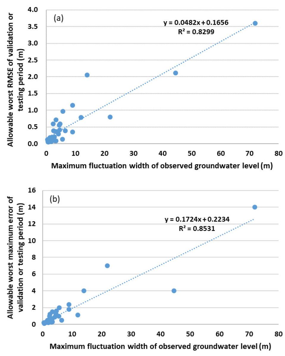
여기에서 Allow.Max.Error는 허용가능한 최대오차(m)이다. 예를 들어, 만약 관측지하수위의 최대변동폭이 10 m인 경우 인공지능 모델의 모의결과에 대한 허용가능한 최대오차는 Eq. (2)에 의해 1.9 m이다.
위에서 추정한 허용가능한 RMSE 산정식(Eq. (1))은 선형회귀식에 의한 평균적인 결과이다. 따라서 추가적인 평가기준을 종합적으로 고려하여 인공지능 모델의 예측성능을 평가하는 것이 필요하며, 기존 연구들의 NSE (Table 1(a))와 R2(Table 1(b))를 사용할 수 있다. Table 1에서 보여주는 바와 같이 기존의 일부 연구들은 NSE 또는 R2를 제시하지 않았다. 따라서 이 누락사항과 이상치의 영향을 고려하기 위해 이 평가지수들의 평균값을 사용하지 않고 중앙값을 사용하였으며 NSE와 R2의 중앙값은 각각 0.849와 0.880이다. 참고로 NSE와 R2의 평균값은 각각 0.806과 0.832이며 따라서 산정한 중앙값이 평균값보다 높은 평가기준이 된다.
종합하면, 인공지능 모델의 지하수위 예측능력은 Eqs. (1) and (2)에 의해 산정된 허용가능한 RMSE 또는 최대오차 이하이거나 NSE ≥ 0.849 또는 R2 ≥ 0.880 인 경우 적합한 것으로 판단된다. 본 연구에서 제시한 NSE값인 0.849는 Moriasi et al. (2007)이 하천유출 모의에 대해 제시한 만족할만한 평가기준인 NSE > 0.50보다 큰 값이므로 강화된 평가기준이라고 할 수 있다.
4. 결 론
본 연구에서는 과거 약 20년 동안 다양한 인공지능 모델들을 활용하여 전 세계의 다양한 수문학적 특성을 가진 지역의 지하수위를 예측한 연구결과들을 종합적으로 분석함으로써 인공지능 모델을 활용한 지하수위 예측결과의 적절성 평가를 위한 기준을 제시하였다. 평가기준 산정 시 국제적으로 검증된 35편의 연구결과를 분석을 위한 자료로 사용함으로써 평가기준 산정결과의 신뢰성을 높였다. 과거 연구결과들을 분석한 결과 관측지하수위의 변동성이 클수록 인공지능 모델에 의한 지하수위 예측오차는 증가하였다. 과거 연구결과들을 활용하여 관측지하수위 최대변동폭 대비 RMSE 및 최대오차의 관계를 분석한 결과 선형회귀식의 R2가 각각 0.8299 및 0.8531을 보여 높은 상관성을 나타내었다. 또한 기존 연구들에서 제시한 지하수위 예측결과에 대한 NSE와 R2를 분석하여 추가적인 평가기준을 제시하였다. 종합하면 인공지능 모델에 의한 지하수위 예측결과는 본 연구에서 제시한 선형회귀식들에 의한 RMSE 또는 최대오차 이하이거나 NSE ≥ 0.849 또는 R2 ≥ 0.880 인 경우 적절한 것으로 판단된다. 본 연구에서 제시한 허용가능한 오차범위는 인공지능 모델을 활용한 지하수위 예측결과의 적절성 판단을 위한 참고자료로 사용할 수 있다. 지하수위 예측결과의 적절성 판단을 위한 허용가능한 오차범위 사용의 실용적인 접근방법은 향후 인공지능을 활용한 지하수위 예측연구에서 제시할 예정이다.
