1. Introduction

Sediment is one of the most difficult water quality constituents to accurately represent in current watershed and river model. Important aspects of sediment behavior within a watershed system include loading and erosion source, delivery of these eroded sediment sources to river, drains and deposition processes. Sediment finally reach to coastal zone by of river path. In connection with the coastal erosion, Phillips has pointed out that rivers are the major source of coastal sediment (Phillips, 1995). The sediment in coastal areas represents evidence of changes from river sediment delivery driven by human or natural impacts. Urbanization affects this equilibrium by decreasing, slowing, and halting the movement of sediment to coastal areas. This is an important issue for many coastal regions around the world (Fernandez et al., 2003; Ferro and Porto, 2000). It is also becoming increasingly obvious that sediment loads in the world’s rivers have been impacted by human development. Although some specific zones have abundant SY data, in practice sediment yield data are very limited in the coastal area due to lack of high cost sediment data collection. This paper synthesizes calculated SY in ungauged basin and newly-derived power function Eq. based on measured SY data. And then this study was conducted to determine the runoff of SY in selected sub-river basin of the Meaho.

Fig. 1.

Location map showing Maeho basins

2. Study area and data collection

South Korea (S. Korea) is surrounded by sea on three sides, with 11,542 km of coastline. Most beaches on the east coast are clayey tidal flats. The tide is semidiurnal with maximum range of about 10 m. On the other hand, most beaches on the east coast are sandy beaches that have been suffering from beach erosion. The coastal region is the most dynamic part of the seascape since its shape is affected by various factors, such as hydrography, geology, climate, and vegetation. Coastal erosion may be caused by natural processes such as waves, currents, and storms as well as human activities such as land reclamation, recreation at beaches, and construction of infrastructure in coastal areas (Rosati, 2005).

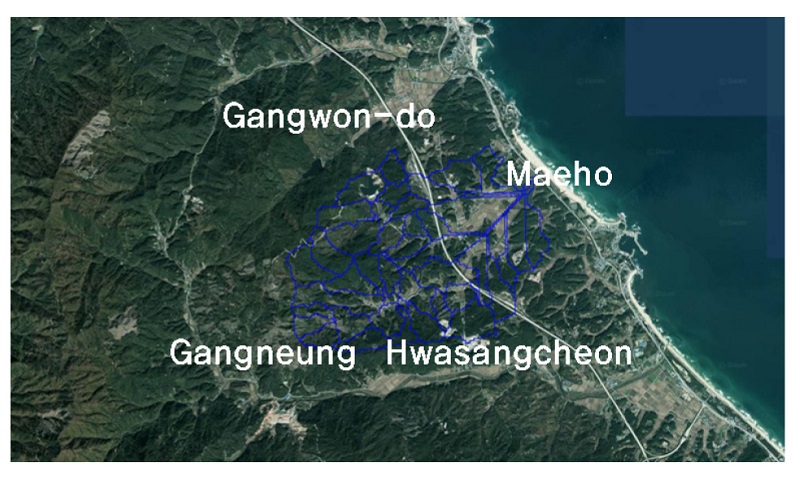
The study area is located on the East coastal side of S. Korea, having 8.2km² of basin as shown in Fig. 1. The Maeho formed from lagoon lies to the end of basin. The present investigations were conducted on the East Sea of S. Korea between both headlands. The coast has a flat slope (1/200) with a narrow beach that ranges from 5 m to 75 m wide. The annual mean rainfall is 1,200 mm, which varies by typhoon. Since 1998, rapid urbanization due to increased population caused intensive construction of buildings, roads and other infrastructures very close to the coastal area. The impacts of urbanization on the coastal area were reviewed by various researchers (Fu et al., 2006; Jain and Kothyari, 2000). Attacks from typhoons sometimes caused a great deal of damage to the region.

In order to analyze the characteristics of soil erosion within the basin and the cause of SY, a soil erosion model requires information on the digital elevation model (DEM), soil, and land cover. To determine the geomorphological character-istics, we developed a triangle irregular network (TIN) using a 1:5,000 scale digital topographic map crafted by the National Geographic Information Institute (NGII). Using the TIN, a 10 m resolution DEM was developed because it is closest to the typical Revised Universal Soil Loss Equation (RUSLE) resolution of 22 m. The land cover of the 1980 and 2005 data was processed using 30 m resolution LANDSAT satellite images by Water Management Information System (WAMIS).

3. Methodology

3.1 Soil erosion

RUSLE is used as a soil erosion model to estimate the amount of soil erosion from basins (Kothyari and Jain, 1997). As the theoretical basis of RUSLE has been clearly reported elsewhere (Lee and Kang, 2014), we provide here only a brief description of the model. In the RUSLE, the amount of soil loss is a product of five factors representing the rainfall and basin characteristics, as follows;

 (1)

where, is the gross amount of soil erosion in cell (t ha^-1 year^-1); R is the rainfall erosivity factor (MJ mm ha^-1 h^-1 year^-1); K is the soil erodibility factor (Tons ha h ha^-1 MJ^-1 mm^-1); LS represent slope length and slope steepness (dimensionless); C is the cover management factor (dimensionless); and P is the supporting practice factor (dimensionless).

R is generally calculated from an annual summation of rainfall data using rainfall energy over 30-min duration. On annual basis, the EI30 value as an erosivity factor is the sum of values over the storms in an individual year. The erosivity of rainfall varies greatly by location because of the effects of elevation in rainfall. Wischmeier and Smith (1978) observed that there's a high correlation between rainfall kinetic energy and its maximum intensity, EI30 and the amount of soil eroded. Erosivity factor is an indication of the two most important characteristics of a storm determining its erosivity: amount of rainfall and peak intensity sustained over an extended period.

Some researchers evaluated the erosivity and developed statistical relationship between R-factor and the total annual precipitation (Pal et al., 2012). As there are limited meteoro-logical stations in mountainous basin, information on rainfall amount and pattern needs to be assumed based on neighboring stations (Lee and Kang, 2013). The rainfall information available represents point data, and this has to be extrapolated in terms of spatial distribution, using the Arc GIS contouring function. In this study, the Eq. (2), developed by Korea Institute of Construction Technology KICT (1992), was used for computing the R factor as:

 (2)

where, P_r is the average annual precipitation of the study area.

The erodibility of a soil K is an expression of its inherent resistance to detachment and transport by rainfall (Wischmeier et al., 1971). It is determined by the cohesive force between the soil particles. Soil erodibility may vary depending on soil characteristics, such as particle distribution, soil structure, and organic matter, etc. The formula for soil erodibility (Kamaludin et al., 2013) is as follows:

                                           (3)

where, OM is organic matter (%), N1 is clay+very fine sand (0.002-0.125 mm), N2 is clay+very fine sand+sand (0.125-2 mm), SS is soil structure code, and PP is profile permeability class (Wischmeier and Smith, 1978).

Korean National Academy of Agricultural Science published the soil map with 1:50,000 scales (KNAAS, 2014). Based on this map, a digital soil map was produced with the ArcGIS coverage of the 1:25,000 scales. Soil classification in study area was divided into 59 types of total 390 soil types.

LS are the slope length and gradient factor. The slope length and slope steepness can be used in a single index, which expresses the ratio of soil loss as defined by Wischmeier and Smith (1978) as:

 (4)

where, X is the slope length (m), m is slope length exponent, and S is slope gradient (%). In order to calculate X value, Flow Accumulation was derived from DEM after conducting Fill and Flow Direction processes in ArcGIS. The vegetation cover factor C represents the ratio of soil loss under a given vegetation cover as opposed to that on bare soil. The vegetation cover intercepts raindrops and dissipates its kinetic energy before it reaches the ground surface (Renard et al., 1997). The relative impact of management options can easily be compared by making changes in the C factor which varies from near zero for well protected land cover to one for the barren areas (Lee and Lee, 2006). The effect of contouring and tillage practices on soil erosion is described by the support practice factor P within the RUSLE model (Renard et al., 1997). Wischmeier and Smith (1998) defined the support practice factor P as the ratio of soil loss with a specific support practice to the corresponding soil loss due to up and down cultivation. If there are no support practices, the P factor is 1.00. Contemporary agricultural practices consist of up and down tillage without the presence of contours, strip cropping, or terracing. The P factor depends on the conservation measure applied to the study area. In this study, the factors C and P were applied on the basis of KICT (1992) classification.

3.2 River sediment yield model

SY is the amount of solid particles that is delivered to the outlet of the basin. SY at a mouth of the basin is calculated by multiplying gross erosion above that point by a SDR. The SY load from each measurement can be derived as:

 (5)

where, is suspended sediment load (t/day), is water discharge (m³/s), is sediment concentration (mg/l)

Calculating the annual sediment load of a river can be quite straightforward, if discharge and sediment concentration are measured at closely spaced intervals, particularly during floods. In most cases, however, a continuous record of sediment concentration is not available, and indirect methods must be utilized using a sediment rating curve (SRC). The SRC is a widely adopted method for estimating sediment concentration and load (Yekta et al., 2010). As sediment concentration and load often vary over several orders of magnitude, the SRC is generally established by a power function (Lu and Siew, 2005) that relates available sediment load () to water discharge ():

 (6)

where, a is regression constant and b is slope by regression analysis.

3.3 Review of sediment delivery ratio

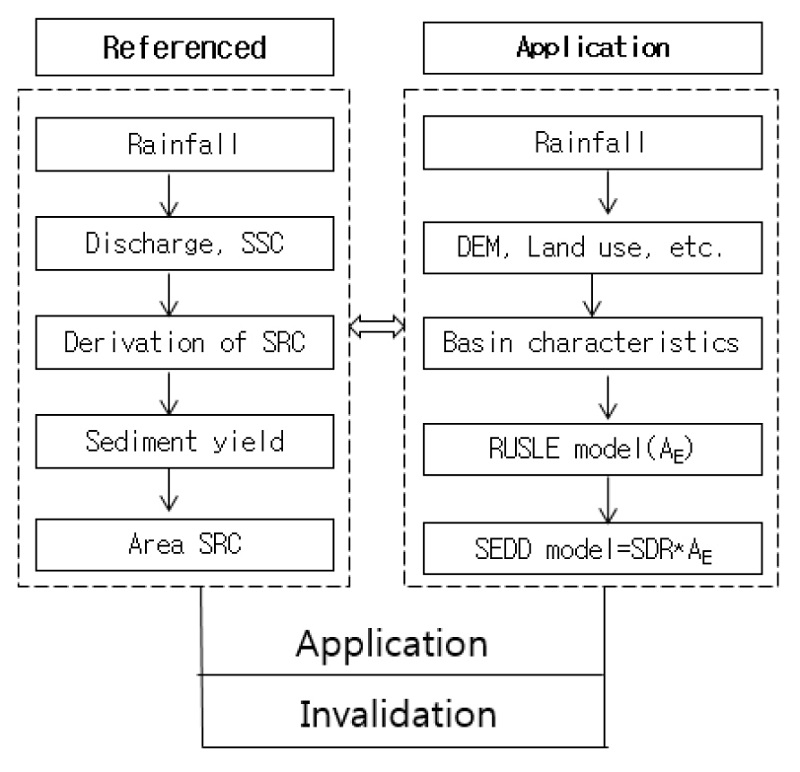
The SDR is the ratio of SY at the outlet, over the total volume of produced sediment using Eq. (5) in the drainage basin. It is well known that the SDR is related to basin size, i.e. it decreases with the size of basin. There are some methods to estimate SDR, namely an observed SRC model linking RUSLE, and a combination of the SEdiment Delivery Distribution (SEDD) model and RUSLE model (Lee and Kang, 2014). The SDR values can be assessed with GIS- based spatially distributed sediment models using field experimental data.

3.3.1 SDR model coupling RUSLE and SRC

RUSLE is a basin model; thus it cannot be directly used to estimate the amount of sediment reaching downstream areas, because some portion of the eroded soil may be deposited while traveling to the watershed outlet or the downstream point of interest (Neibling and Foster, 1977). To account for these processes, the SDR for a given watershed should be used to estimate the total sediment transported to the watershed outlet. The SDR can be expressed as follows:

 (7)

3.3.2 SEDD model

Empirical Equations for SDR are usually based on variables, such as basin area, slope and land cover (Ferro and porto, 2000). For example, Kothyari and Jain (1997) estimated the SDR values from the watershed area, relief ratio and average runoff curve number value. They applied a lumped approach, but improved this by division of the modeled basin into smaller watersheds. According to some authors (Mutua and Klik, 2006), the coefficient, which is a measure of the probability that the eroded particles are transferred from the morphological unit under consideration to the nearest stream reach, can be generalized as follows:

 (8)

where, is basin specific parameter depends on morpho-logical data, is travel time (hr) of overland flow from the overland cell to the nearest channel cell down the drainage path.

If the flow path from cell i to the nearest channel traverses Np cells, then the travel time from that cell is calculated by adding the travel time for each of the Np cells located along the flow path. is the length of segment i in the flow path (m), and is equal to the length of the side or diagonal of a cell, depending on the flow direction in the cell. is the flow velocity for the cell (m/s). The flow velocity is considered to be a function of the land surface slope and the land cover characteristics, i. e. . If is the amount of soil erosion produced within the cell of the basin estimated using Eq. (1), then the SY for the basin, SY, is obtained, as below:

 (9)

where, n is the total number of cells over the basin. Since the SDR of a cell is hypothesized as a function of travel time to the nearest channel, this implies that the gross erosion in that cell multiplied by the SDR value of the cell becomes the SY contribution of that cell to the nearest stream channel. The SDR values for the cells marked as channel cells are assumed to be unity. SY modeling is a more complicated and time- consuming process, since the RUSLE method cannot drive the SY directly. In order to estimate the SY, then we combine the RUSLE and SDR model, using the Model Builder (MB) in the ArcGIS environment. Simulated SY was validated with observed one as shown in Fig. 2.

Fig. 2.

Model validation process between calculated and observed sediment yields using model builder of ArcGIS

4. Results

4.1 Soil erosion

In order to calculate SDR by modeling, the relationship between soil loss and SY needs to be determined. The annual soil erosion from each identified grid of the basin was computed by integration of the RUSLE erosion factors, namely R, K, LS, C and P of RUSLE. The values of the RUSLE parameters were integrated in ArcGIS, using a Raster Calculator to form a composite map denoting gross soil erosion, based on 30 m DEM. Land use data of 30 × 30 m, provided by the Water Management Information System in 1980and 2015, was reclassified to create a new map with the following categories: (a) water, (b) urban, (c) barren, (d) wetland, (e) pasture, (f) forest, (g) paddy farming, and (h) field crop area. The soil classification map of the study area was divided into 59 soil types such as Afa, Ana, Apa, Rea, Maa, Ro, etc. In 1973, the NAAS published the soil map at a scale of 1:50,000. Based on this paper map, a digital soil map was produced with the ArcGIS coverage of a 1:25,000 scale. Rainfall erosivity is determined by climatic data. For calculating R factors in the study basins, we used an annual average value using the isohyetal method (Lee and Kang, 2013) based on 59 meteorological observation stations.

Changes occurring in the values of the factor C due to crop growth over such a small duration were neglected (Mutua and Klik, 2006). In this study, the factors C and P were applied on the basis of KICT (1992) classification.

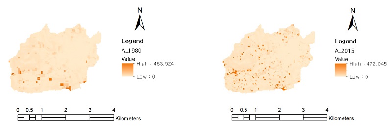
Computed values of average annual erosions of Maeho basin are presented in Fig. 3. The annual average soil erosion for the Maeho basin ranged from 320 to 333 tons/km²/yr for the two years of 1980 and 2015. These values are slightly lower than those obtained by Lee and Kang (2014), probably as a consequence of using a DEM to calculate length-slope factors.

Fig. 3.

Soil erosion potential map of Maeho basin

4.2 Sediment load to ungauged coastal basin and validation

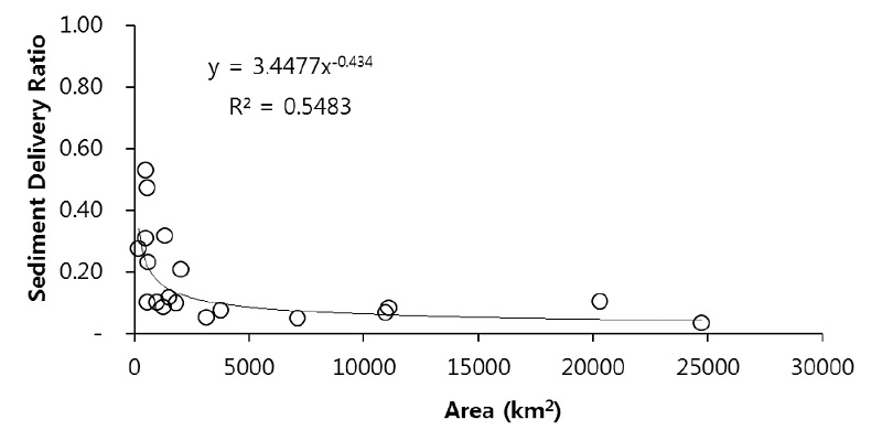
In order to estimate the variation of SY in the ungauged coastal regions, SDR was derived from Eq. (8). SY is the function of SDR and Soil erosion. It is well known that an inverse relationship exists between SDR and the basin area. SDR generally increases with decreasing basin size. The SDR in the field approaches 100% for small and urbanized basins (Lee and Kang, 2014) as shown in Fig. 4.

Fig. 4.

Comparison of different relations between SDR and basins

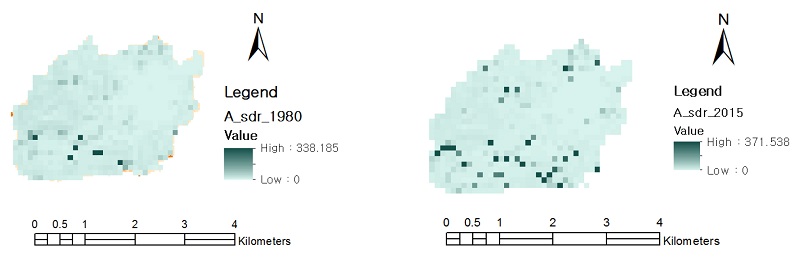
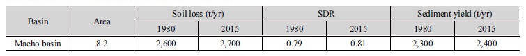
According to preceding research the steepest areas of a basin are the main sediment producing zones, and since average slope decreases with increasing basin size the sediment production per unit grid decreasing too. Large basins also have more sediment storage sites located between sediment source area and the basin outlet (Kang, 2015). After the values of RUSLE and SDR were derived, SY was calculated using Eq. (9). As shown in Fig. 5, SY was calculated to range from 2,300 to 2,400 t/ha for the ungauged Maeho basin, during two years of 1980 and 2015. And the computed SY in the study basin for the two years are summarized as shown in Table 1.

Fig. 5.

Sediment yield map of Maeho basin

Table 1. Annual sediment transport for ungauged coastal basin

Otherwise, in other to estimate annual SY, a SRC was derived as a linear regression using Eq. (5), on the basis of reference data. As sediment concentration and load often vary over several orders of magnitude, the SRC is generally established by a power function (Lee and Kang, 2014) that relates available sediment load (Q_S) to water discharge (Q_W):

 (10)

where, is regression constant and is slope by regression analysis.

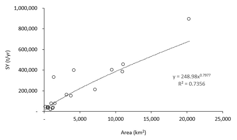
Fig. 6 shows discharge of SY with basin area using published data. If the basin size of the Maeho is 8.2 km², the SY may be 1,333 (t/yr) by power function of Eq. (10), approximately. The SY calculated from the Eq. (10) has a lower value than the modeled owns. We can estimate that it is because of a long period (December to next March) of the whole year has a melting season, with little or no rainfall in S.Korea. Over 80% of total SY is concentrated on wet monsoon periods and it will reduce the SY to rivers.

Fig. 6.

Relation of SY and area for the reference areas

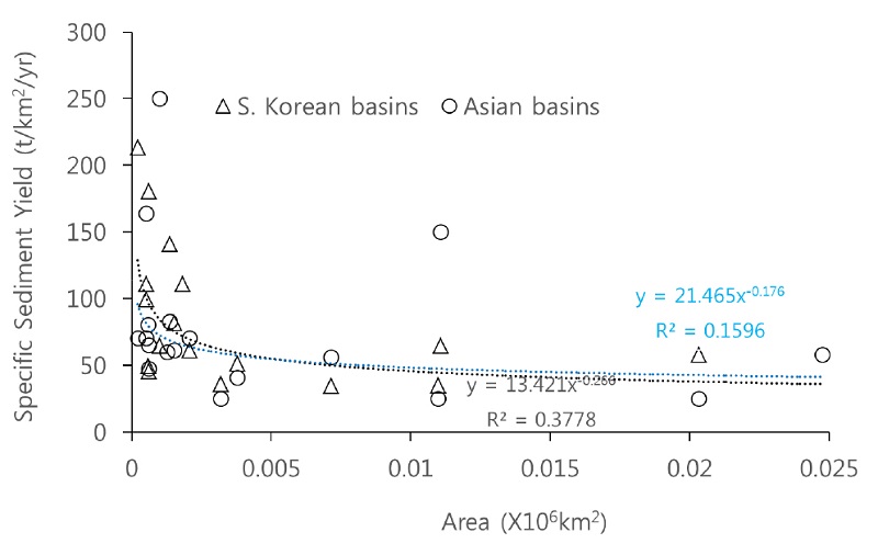
The Specific Sediment Yield (SSY) of 17 rivers in Korean basins ranged from 34 to 213 t km^-2yr^-1 (Lee and Kang, 2014). These SSY values are similar trend to that of a previous result obtained by Milliman and Syvitski (1992) for 22 Asian river basins from 25 to 250 t km^-2yr^-1 as shown in Fig. 7.

Fig. 7.

Calculated specific sediment yield based on data in Milliman and Syvitski (1992) and in addition Lee and Kang (2014)

5. Conclusions

The SY, especially in coastal areas, is too sensitive to readily obtain data. Their data has been scarcely used, because its conventional measurement methods are expensive and time-consuming. In this paper, a theoretically based relationship for evaluating the soil loss and SDR is proposed to estimate SY in an ungauged basin. Soil erosion in the individual cells of the basin was determined using the RUSLE. The value of SDR was calibrated comparing the calculated SY for the study basins and similar observed basins, as defined by Eq. (8). The annual SDR at the outlet of the basin was estimated in the range from 0.75 to 0.81 for the Maeho basin. The calculated SSY ranged from 271 to 296 t/km²/yr for the Maeho. The method depends on calibration against a record of existing conditions and hence it can be used for the estimation of SY in other such ungauged basins which have similar hydro-meteorological and land cover conditions.