

1. Introduction
2. Models and Data Pre-Processing Approach
2.1 Gated recurrent unit (GRU)
2.2 Generalized regression neural networks (GRNN)
2.3 Random forests (RF)
2.4 Discrete wavelet transform (DWT)
2.5 Evaluation of independent and two-stage hybrid models’ performance
3. Study Boundary and Data Information
4. Results and Discussion
4.1 Dosan station
4.2 Hwangji station
4.3 Discussion
5. Conclusions
1. Introduction
Water quality can be specified as the biological, chemical, and physical aspects of corresponding water of rivers, reservoirs, and oceans (Ahmed and Shah, 2017; Kim et al., 2020). The water quality indicators can be involved the several items including water temperature (WT), electrical conductivity (EC), biochemical oxygen demand (BOD), dissolved oxygen (DO), the potential of Hydrogen (pH), turbidity (TU), chemical oxygen demand (COD), suspended solids (SS), total organic carbon (TOC), total nitrogen (T-N), total phosphorus (T-P), and chlorophyll-a (CHA) and so on. Also, their assessment can be very important for the critical management of different water resources systems (Khaled et al., 2017; Kim et al., 2020).
BOD concentration has been accepted as a confirmation of river water pollution by the U.K. Royal Commission on River Pollution since 1908 (Royal Commission on Sewage Disposal, 1908). From the commission meeting, the five-day term at a 20 Celsius degree (℃) was defined and handled to estimate BOD5 concentration. In USA, the American Public Health Association Standard Methods Committee (APHASMC) classified BOD concentration as a quotation to evaluate the natural pollution of water since 1936 (Jouanneau et al., 2014). In addition, BOD concentration can be proposed as the requirement of DO concentration to lessen the natural material of water at the addressed temperature (Raheli et al., 2017; Tao et al., 2019).
Measurement of water quality indicators is categorized as three divisions including on-site measuring classification (e.g., WT, DO, pH, and TU), laboratory-based analysis classification (e.g., COD, SS, TOC, T-N, T-P, and CHA), and incubated-based analysis classification (e.g., BOD). Therefore, BOD concentration can be computed employing the amount of oxygen concentration consumed per liter of sampling data based on the five-day term at a 20 Celsius degree (℃). Zou et al. (2007) explained that the traditional approaches of water quality indicators required much time and effort to overcome the addressed prediction problems. Also, Ay and Kisi (2012) demonstrated that BOC concentration was one of important water quality indicators for conservation and maintenance of ecosystems in rivers.
To beat the drawbacks of traditional approaches for the prediction problems of water quality and hydrology, deep learning and machine learning approaches have been surveyed and published the numerous documents since two thousand (Zhang et al., 2002; Diamantopoulou et al., 2007; Dogan et al., 2009; Kim, 2000, 2011; Kim and Kim, 2007; Kim et al., 2009, 2012; Li et al., 2019; Zounemat-Kermani et al., 2019; Kim et al., 2021). Among the diverse deep learning and machine learning approaches, a few particular mechanisms have been employed to predict BOD concentration (Emamgholizadeh et al., 2014; Noori et al., 2015; Ahmed and Shah, 2017; Khaled et al., 2017; Raheli et al., 2017; Ahmadi et al., 2018; Tao et al., 2019).
Granata et al. (2017) predicted the water quality indicators including BOD, COD, total dissolved solid (TDS), and total suspended solids (TSS) concentrations utilizing the support vector regression (SVR) and regression tree (RT) models in USA. Solgi et al. (2017) predicted BOD concentration employing the hybrid SVR and adaptive neuro-fuzzy inference system (ANFIS) models in the Karun River, Iran.
Though diverse deep learning and machine learning approaches have been employed for predicting specific water quality indicator in rivers, novel approaches are required to enhance the prediction accuracy of BOD concentration. In this investigation, a novel two-stage hybrid paradigm (i.e., wavelet-based gated recurrent unit, wavelet-based generalized regression neural networks, and wavelet-based random forests) which includes the combination of data pre-processing (i.e., discrete wavelet transform), deep learning, and machine learning approaches (i.e., gated recurrent unit, generalized regression neural networks, and random forests), provides the capability and efficiency for the solution of complicated and high nonlinear problems. Within the range of our experience and recognition, the novel two-stage hybrid paradigm has not been employed for this argument.
This investigation demonstrates the accuracy and capability of DWT-GRU, DWT-GRNN, and DWT-RF models for predicting BOD concentration in South Korea. The performance of addressed models are evaluated and compared to the independent models based on three statistical indices (i.e., RMSE, NSE, and CC) and graphical support (i.e., scatter diagram and Taylor scheme). This investigation is classified as follows: The chapter two supplies the addressed models and data pre-processing approach, respectively. Study boundary and data information are suggested in the chapter three, and chapter four illustrates results and discussion. Finally, conclusions are summarized in the chapter five.
2. Models and Data Pre-Processing Approach
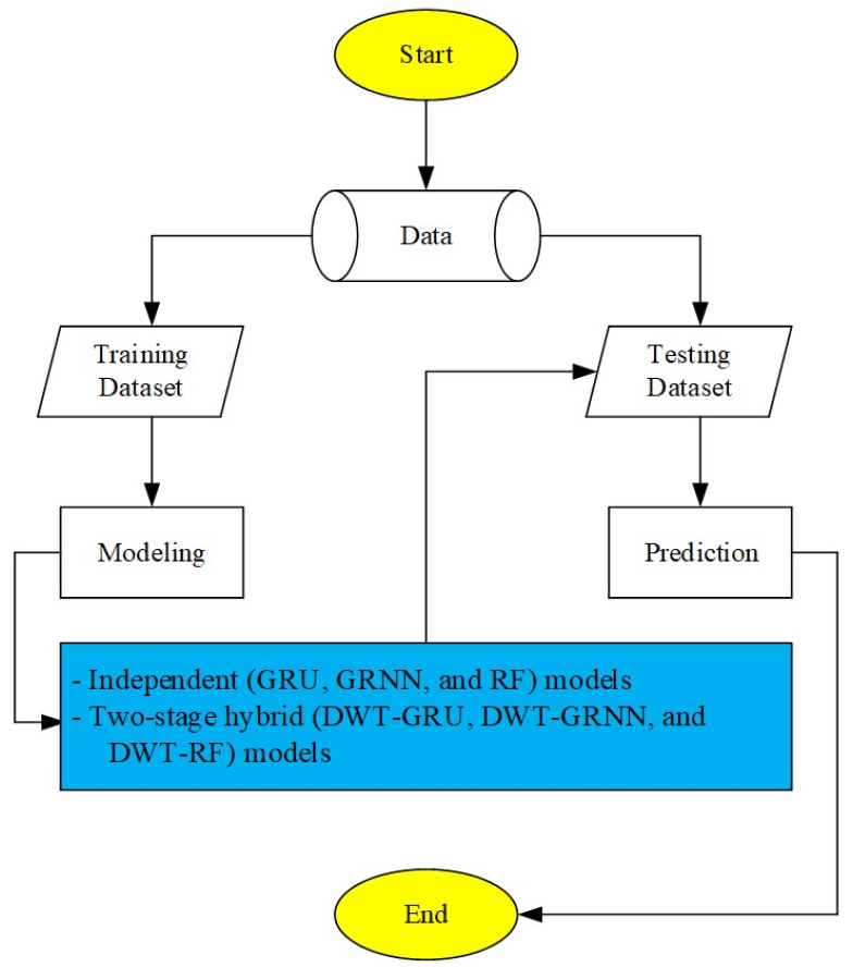
The addressed models employed in this investigation are deep learning (i.e., GRU) and machine learning (i.e., GRNN and RF) models, respectively. In addition, the implemented data pre-processing approach is the discrete wavelet transform (DWT) method. Subsequent section expressed the addressed models and data pre-processing approach. It can be found from Fig. 1 that the universal modeling and prediction process of implemented investigation is emphasized.
2.1 Gated recurrent unit (GRU)
Gated recurrent unit (Fig. 2) is an advanced report of long short-term memory (LSTM) model implemented by Cho et al. (2014). The GRU model is an improved approach employing the gating mechanism based on the LSTM model, and reduces the management of memory cells compared to the LSTM model (Yang et al., 2020). The GRU model restricts the signal signs to two gates. Revising the gate decides how frequently the device changes its arrangement or information. The reset gate determines to combine the current arrangement information with the historical memory. Also, adjustment of parameters are utilized in the GRU model arrangement. The computational processes for the update gate, reset gate, input gate, and standard GRU model are represented by the following Eqs. (1)~(4).
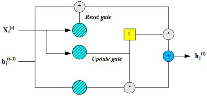
where is the input for time series (t), (WZ, WR, WI) and (UZ, UR, UI) are the weight matrices of input and hidden layers for different gates, is the output of update gate for time series (t), is the output of reset gate for time series (t), is the output of input gate for time series (t), is the output of GRU cell for time series (t), is the output of short-term state cell for time series (t-1), is the hyperbolic tangent function, and are the sigmoid functions, and * is the Hadamard product.
2.2 Generalized regression neural networks (GRNN)
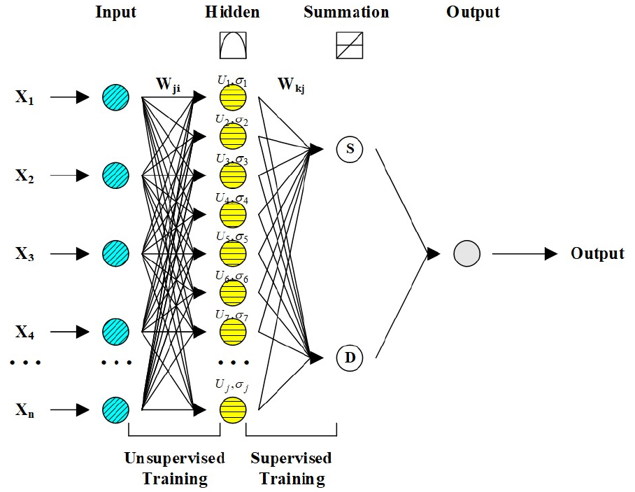
Generalized regression neural networks (Fig. 3) expresses a shifted strategy of radial basis function (RBF) (Specht, 1991). The input, hidden, summation, and output layers are the core pattern of design for the GRNN model’s policy. The equivalent neurons of input, hidden, and summation layers are completely connected, whereas the neuron of output layer is correlated with only a few neurons equivalent to the summation layer. Two strategies of neurons including different summation neurons and only one division neuron aggregate the summation layer. The number of summation and output neurons is identical. The division neuron, however, implements the inclusion of weighted designated signals from the neurons of hidden layers instead of a transfer function. Each neuron from output layer is correlated with the summation and division neurons equivalent to the summation layer. In addition, the connection weights from the summation to the output layers are not constructed. The computation of each neuron equivalent to the output layer is evaluated employing dividing the output signals from the summation neuron by the output neuron from division neuron equivalent to the summation layer (Kişi, 2006; Kim and Kim, 2008; Ladlani et al., 2012; Li et al., 2014; Ahmadi et al., 2019).
2.3 Random forests (RF)
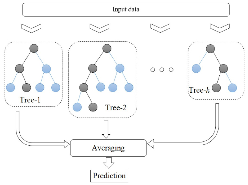
Random forests (RF) (Fig. 4) which collects the decision trees that evolve in parallel, was inaugurated by Breiman (2001). The prediction of trees are incorporated to make the general prediction of forest trees. A RF model resembles a Treeboost model (Friedman, 2002) because the RF and Treeboost models employ many trees similarly. However, the core difference between both models is that the trees in the Treeboost model are evolved in sequence such that the output of one tree is supplied to the next tree, whereas a RF model collects the independent trees that are evolved in parallel pattern (Simard et al., 2000; Zounemat-Kermani et al., 2017; Alizamir et al., 2021). The RF model employs a randomized and separated methodology for providing many different unpruned decision trees to each neuron. Therefore, the results of approximated trees makes a more stable and flexible architecture for accomplishing accurate and efficient prediction. The majority decision or arithmetic average is examined for aggregating prediction (Breiman, 2001).
2.4 Discrete wavelet transform (DWT)
Discrete wavelet transform (DWT) approach has been approved as one of multi-resolution signal procedure approaches (Kim et al., 2016; Seo and Kim, 2016; Seo et al., 2015, 2016, 2018). The data of original time series can be divided into diverse frequency element including an approximation and multiple details employing the DWT approach. If X = is a time series data, the J0-level DWT approach of X provides W (i.e., DWT coefficients) employing an orthonormal transform (Percival and Walden, 2000).
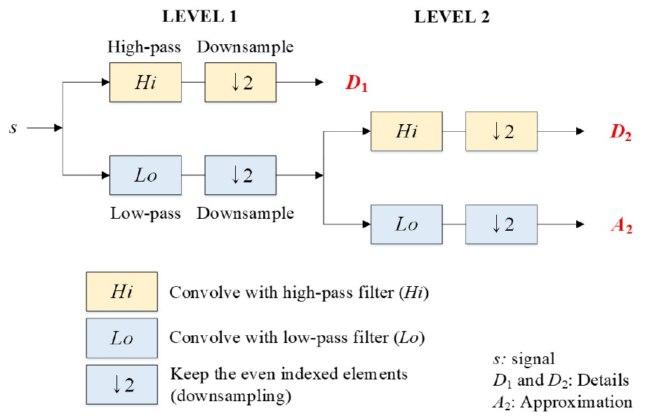
In fact, the DWT approach can be performed utilizing the Mallat algorithm (Mallat, 1989). The core point of Mallat algorithm is two-channel filters which make up high-pass (wavelet) filter and low-pass (scaling) filter . The main system is comprised of circular filtering and downsampling. Percival and Walden (2000) explained that the wavelet and scaling coefficients for the jth decomposition level can be defined as following Eq. (5).
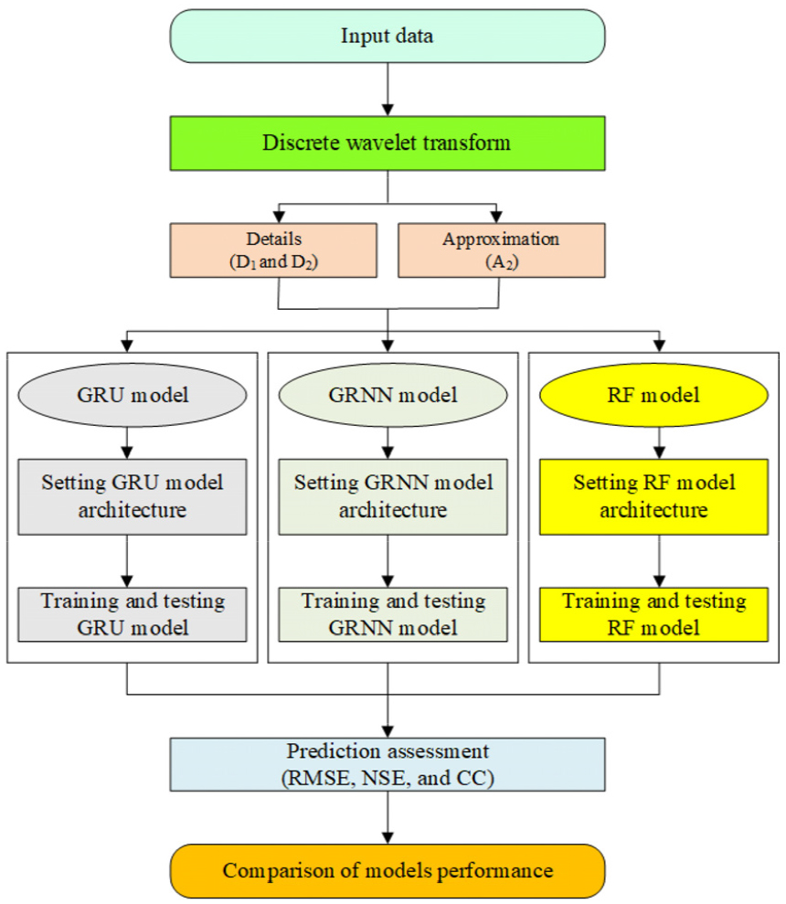
where Wj,t and Vj,t are the elements of Wj and Vj, respectively. A schematic diagram for two-level DWT approach can be found in Fig. 5. In this investigation, two details (D1 and D2) and an approximation (A2) are generated from an original time series. Fig. 6 shows the flowchart for developing the DWT-GRU, DWT-GRNN, and DWT-RF models.
2.5 Evaluation of independent and two-stage hybrid models’ performance
To evaluate the independent and two-stage hybrid models’ performance, diverse and different statistical indices were implemented. The difference between observed and predicted BOD concentration can be computed by utilizing root mean square error (RMSE) (Willmott and Matsuura, 2005) index. RMSE = 0 indicates the accurate computation for predicting BOD concentration. RMSE index (i.e., see the Eq. (6)) must be applied for model evaluation (Deo et al., 2019). The Nash-Sutcliffe efficiency (NSE) (Nash and Sutcliffe, 1970) index can judge the models’ efficiency between observed and predicted BOD concentration. The perfect model (i.e., computed error variance = 0) shows the NSE index equals one. In case of the predicted BOD concentration when the computed error variance is larger than the observed variance, the NSE < 0 occurs. Garrick et al. (1978) investigated that NSE index (i.e., see the Eq. (7)) can be significantly accurate value (e.g., over 0.8) for poorly-matched models, while the best-matched models cannot yield accurate values. Correlation coefficient (CC) index is explained as the correlation between observed and predicted BOD concentration. When CC index indicates zero value, BOD concentration cannot be predicted, while the prediction of BOD concentration can be accomplished perfectly when CC index shows one value (Zounemat-Kermani et al., 2019; Kim et al., 2020). CC index can be computed employing Eq. (8).
where BODobs and BODpre are the observed and predicted BOD concentrations, obs and pre are the observed and predicted mean BOD concentration, and n is total number for data available.
3. Study Boundary and Data Information
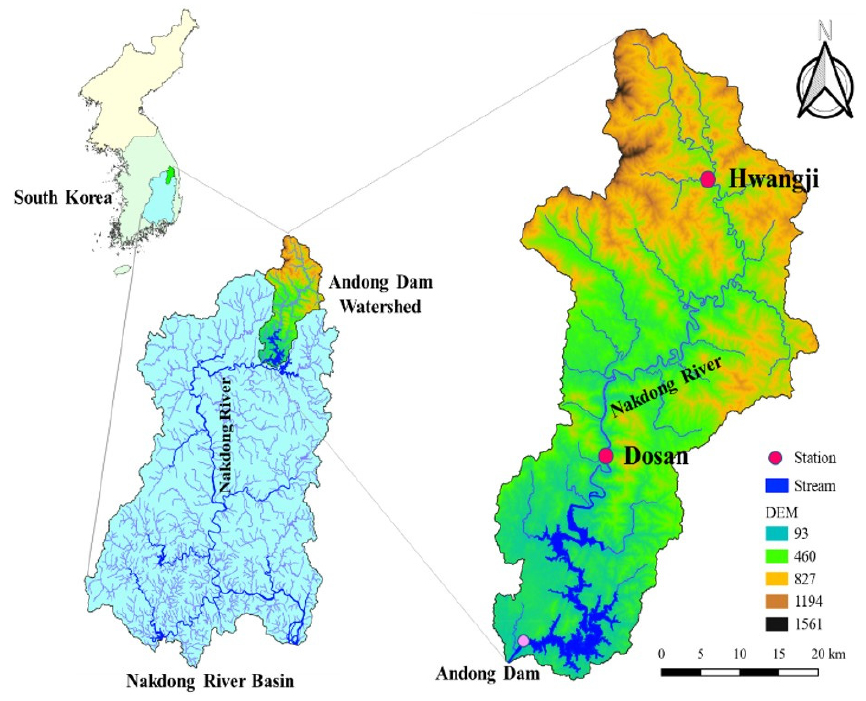
In this investigation, Dosan (latitude 36°77' 24'' N; longitude 128°89' 04'' E) and Hwangji (latitude 37°06' 74'' N; longitude 129°05' 07'' E) stations were chosen to predict BOD concentration in the upper Nakdong River basin, South Korea. The analysis of water quality and quantity indicators was accomplished based on eleven physical and chemical characteristics including BOD, TOC, T-P, T-N, COD, SS, WT, DO, EC, pH, and water discharge (DIS). Only DIS represents water quantity indicator. Fig. 7 shows the schematic maps of Dosan and Hwangji stations.
The historic data (January 2008 - December 2020) with the irregular measured periods for water quality and quantity indicators can be downloaded and collected directly from the web-based information system of National Institute of Environmental Research (NIER) (http://water.nier.go.kr) which is managed and operated by the Ministry of Environment (ME), South Korea. Also, the perfect data were separate into training and testing datasets. The training data included 80% (N = 407 for Dosan and N = 398 for Hwangji) of perfect data, and the testing data utilized the remnant 20% (N = 101 for Dosan and N = 99 for Hwangji), respectively. Table 1 provides basic statistical properties of water quality and quantity indicators.
On July 15, 2020, the Ministry of Environment (ME) announced that it would prepare a target of water quality indicator for the border areas of water pollution control system that each provincial government in the Han River and Nakdong River water system must achieve by 2030. Also, the target of water quality indicator in the Nakbon-A station (i.e., border area of local water pollution control system including Dosan and Hwangji stations in the Nakdong River) to be achieved by 2030 is to reduce BOD concentration by 1.40 (mg/L) on average (ME, 2020). Table 1 demonstrates, therefore, the stable and acceptable ranges of BOD concentration on average for Dosan (0.91 mg/L) and Hwangji (1.18 mg/L) stations compared to the Nakbon-A station.
For the advanced understanding of individual water quality and quantity indicators affecting on the BOD concentration, the correlations between corresponding input indicators and BOD concentration were computed and listed in table 2. It can be found that COD and TOC indicators provided the significant correlations on BOD concentration at both stations. In this investigation, CategoryⅠ(i.e., on-site measuring classification) includes pH, EC, DO, and WT water quality indicators which can analyze the sample data collected from the on-site measuring field directly. CategoryⅡ, however, demonstrates SS, COD, T-N, T-P, TOC (i.e., laboratory-based analysis classification), and BOD (i.e., incubated-based analysis classification) which can compute the sample data gathered from the laboratory facility indirectly. Finally, Category Ⅲ expresses the water quantity indicator such as DIS.
Table 1.
Statistical properties of water quality and quantity indicators
Table 2.
Computation of correlations between corresponding input indicator and BOD concentration
4. Results and Discussion
This investigation implemented various water quality and quantity indicators to predict BOD concentration at Dosan and Hwangji stations, South Korea. As clarified previously, the evaluation for performance of independent and two-stage hybrid models to predict BOD concentration is the core concept of this investigation.
A few ones (e.g., pH, EC, DO, and WT) among water quality indicators can be directly measured using the specific monitoring instrument. Also, some of them (e.g., SS, COD, T-N, T-P, and TOC) can be measured indirectly based on the laboratory-based analysis, and required a certain level of time. However, BOD, one of water quality indicators in total water pollution management of Four River, South Korea, can be measured by incubating at 20 Celsius degree (℃) during five-day indirectly (Jouanneau et al., 2014). Because the aim of this investigation is explained as the prediction of BOD concentration utilizing deep learning and machine learning approaches directly, it can save the time and activity to incubate BOD in the laboratory facility.
Different associations of water quality and quantity indicators were implemented as a concept of input combination to select the best input combination at both stations. Therefore, the independent and two-stage hybrid models were developed for predicting BOD concentration by applying the diverse input combinations. Since the COD and TOC indicators were selected as the fundamental water quality ones at both stations, this investigation specified the combination of two addressed water quality indicators as Division 1. Diverse input combinations of water quality and quantity indicators to predict BOD concentration are implemented in Table 3 where all developed model were classified into five divisions (i.e., Divisions 1-5).
Table 3.
Diverse input combinations of independent and two-stage hybrid models
4.1 Dosan station
4.1.1 Independent models
The results of three statistical indices for different independent models are arranged in Table 4 at Dosan station. It can be noticed from Table 4 that results of RF1 model (CC = 0.777, NSE = 0.603, and RMSE = 0.212 mg/L) were better than those of GRU1 and GRNN1 models during testing step based on Division 1. In Division 2, the RF2 model (CC = 0.931, NSE = 0.857, and RMSE = 0.127 mg/L) was superior to the GRU2 and GRNN2 models. Also, the RF3 model (CC = 901, NSE = 0.809, and RMSE = 0.147 mg/L) outperformed the GRU3 and GRNN3 models in Division 3 during testing step. In addition, comparison of independent models in Division 4 suggested that the RF4 model (CC = 0.937, NSE = 0.870, and RMSE = 0.122 mg/L) prevailed the GRU4 and GRNN4 models clearly during testing step. Finally, the RF5 model (CC = 0.938, NSE = 0.875, and RMSE = 0.119 mg/L) was more precise than the GRU5 and GRNN5 models during testing step in Division 5.
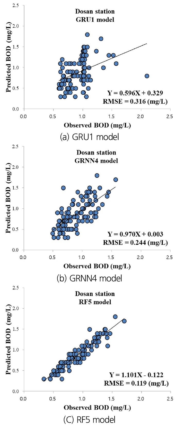
Acknowledging the outstanding models from all Divisions 1-5, the best performance of independent models (i.e., GRU (Division 1), GRNN (Division 4), and RF (Division 5)) can be identified among various input combinations during testing step. It can be recognized from Table 4 that the optimal architecture of RF5 model provided more precise results than the GRU1 and GRNN4 models during testing step. Therefore, the RF5 model was more authentic than the GRU1 and GRNN4 models for predicting BOD concentration among the optimal independent models at Dosan station.
Table 4.
RMSE, NSE, and CC values for the independent and two-stage hybrid models at Dosan station
To validate the precision of optimal models using graphical support, Figs. 8(a)~8(c) give the scatter diagrams for observed and predicted BOD concentration values using the optimal independent models at Dosan station. The values of RMSE index and linear equations for the optimal independent models were demonstrated for each scatter diagram. It can be noted from RMSE values that a clarified difference can be traced among the GRU1, GRNN4, and RF5 models. Accordingly, the RF5 model performed better than GRU1 and GRNN4 models clearly, whereas the GRU1 model yielded the worst precision at Dosan station.
4.1.2 Two-stage hybrid models
The results of three statistical indices for different two-stage hybrid models are also filed in Table 4 at Dosan station. It can be recognized from Table 4 that results of DWT-RF1 model (CC = 0.936, NSE = 0.860, and RMSE = 0.126 mg/L) were better than those of the DWT-GRU1 and DWT-GRNN1 models during testing step considering Division 1. Based on Division 2, the DWT-RF2 model (CC = 0.952, NSE = 0.885, and RMSE = 0.114 mg/L) was more excellent than the DWT-GRU2 and DWT-GRU2 models. In addition, the DWT-RF3 model (CC = 937, NSE = 0.859, and RMSE = 0.126 mg/L) surpassed the DWT-GRU3 and DWT-GRNN3 models regarding Division 3 during testing step. Furthermore, comparison of two-stage hybrid models in Division 4 implemented that the DWT-RF4 model (CC = 0.945, NSE = 0.869, and RMSE = 0.122 mg/L) dominated the DWT-GRU4 and DWT-GRNN4 models apparently during testing step. Finally, the DWT-RF5 model (CC = 0.960, NSE = 0.897, and RMSE = 0.108 mg/L) was more accurate than the DWT-GRU5 and DWT-GRNN5 models during testing step based on Division 5.
Defending the distinguished models from all Divisions 1-5, the superior performance of two-stage hybrid models (i.e., DWT-GRU (Division 5), DWT-GRNN (Division 4), and DWT-RF (Division 5)) can be described among various input combinations during testing step. It can be perceived from Table 4 that the optimum structure of DWT-RF5 model yielded more accurate results than the DWT-GRU5 and DWT-GRNN4 models during testing step. Therefore, the DWT-RF5 model was more reliable than the DWT-GRU5 and DWT-GRNN4 models for predicting BOD concentration among the optimum two-stage hybrid models at Dosan station.
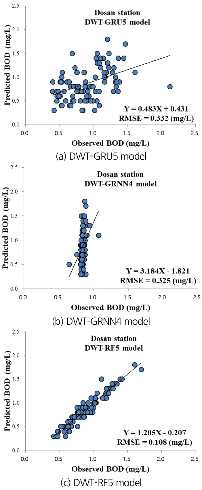
To confirm the accuracy of optimum models using graphical aid, Figs. 9(a)~9(c) give the scatter diagrams for observed and predicted BOD concentration values using the optimum two-stage hybrid models at Dosan station. The values of RMSE index and linear equations for the optimum two-stage hybrid models were displayed for corresponding scatter diagram. It can be judged from RMSE values that a clear difference can be detected among the DWT-GRU5, DWT-GRNN4, and DWT-RF5 models. As a result, the DWT-RF5 model accomplished better than DWT-GRU5 and DWT-GRNN4 models distinctly, while the DWT-GRNN4 model provided the worst accuracy at Dosan station.
4.2 Hwangji station
4.2.1 Independent models
The results of three statistical indices for different independent models are provided in Table 5 at Hwangji station. It can be judged from Table 5 that results of RF1 model (CC = 0.959, NSE = 0.911, and RMSE = 0.269 mg/L) were better than those of the GRU1 and GRNN1 models during testing step based on Division 1. In Division 2, the RF2 model (CC = 0.990, NSE = 0.955, and RMSE = 0.191 mg/L) was superior to the GRU2 and GRNN2 models. Also, the RF3 model (CC = 0.990, NSE = 0.968, and RMSE = 0.163 mg/L) exceeded the GRU3 and GRNN3 models in Division 3 during testing step. In addition, comparison of independent models in Division 4 submitted that the RF4 model (CC = 0.994, NSE = 0.965, and RMSE = 0.170 mg/L) controlled the GRU4 and GRNN4 models clearly during testing step. Finally, the RF5 model (CC = 0.993, NSE = 0.966, and RMSE = 0.168 mg/L) was more correct than the GRU5 and GRNN5 models during testing step in Division 5.
Admitting the magnificent models from all Divisions 1-5, the best performance of independent models can be selected among various input combinations during testing step. It can be classified from Table 5 that the optimal architecture of RF3 model produced more correct results than the GRU4 and GRNN5 models during testing step. Therefore, the RF3 model was more reliable than the GRU4 and GRNN5 models for predicting BOD concentration among the optimal independent models at Hwangji station.
Table 5.
RMSE, NSE, and CC values for the independent and two-stage hybrid models at Hwangji station
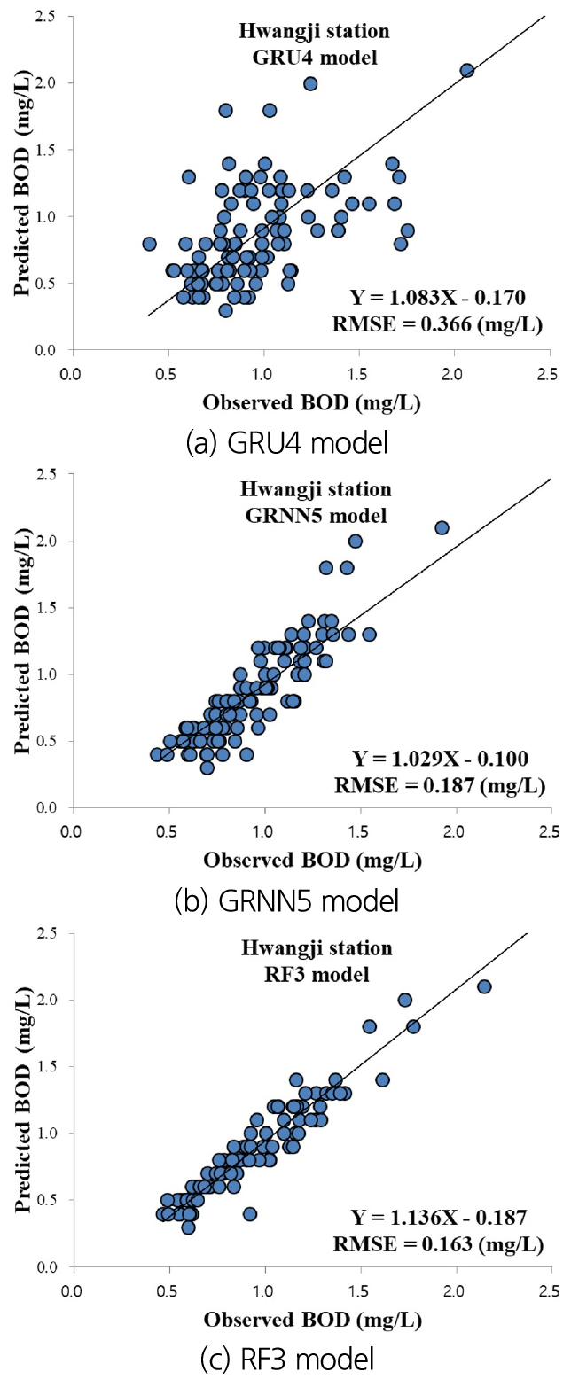
To validate the correctness of optimal models using visual support, Figs. 10(a)~10(c) support the scatter diagrams for observed and predicted BOD concentration values using the optimal independent models at Hwangji station. The values of RMSE index and linear equations for the optimal independent models were indicated for each scatter diagram. It can be proved from RMSE values that a resolved difference can be ascertained among the GRU4, GRNN5, and RF3 models. Accordingly, the RF3 model carried out better than GRU4 and GRNN5 models definitely, whereas the GRU4 model generated the worst correctness at Hwangji station.
4.2.2 Two-stage hybrid models
Also, the results of three statistical indices for different two-stage hybrid models are registered in Table 5 at Hwangji station. It can be perceived from Table 5 that results of DWT-RF1 model (CC = 0.986, NSE = 0.957, and RMSE = 0.187 mg/L) were superior to those of the DWT-GRU1 and DWT-GRNN1 models during testing step reflecting Division 1. Division 2 yielded that the DWT-RF2 model (CC = 0.985, NSE = 0.948, and RMSE = 0.206 mg/L) was more superb than the DWT-GRU2 and DWT-GRU2 models. Moreover, the DWT-RF3 model (CC = 0.981, NSE = 0.938, and RMSE = 0.225 mg/L) outperformed the DWT-GRU3 and DWT-GRNN3 models taking notice of Division 3 during testing step. Furthermore, comparison of two-stage hybrid models in Division 4 achieved that the DWT-GRNN4 model (CC = 0.990, NSE = 0.979, and RMSE = 0.132 mg/L) handled the DWT-GRU4 and DWT-RF4 models obviously during testing step. Finally, the DWT-RF5 model (CC = 0.986, NSE = 0.953, and RMSE = 0.196 mg/L) was more efficient than the DWT-GRU5 and DWT-GRNN5 models during testing step based on Division 5.
Securing the discerning models from all Divisions 1-5, the outstanding performance of two-stage hybrid models can be provided among various input combinations during testing step. It can be understood from Table 5 that the optimum structure of DWT-RF1 model produced more efficient results than the DWT-GRU4 and DWT-GRNN4 models during testing step. Therefore, the DWT-RF1 model was more stable than the DWT-GRU4 and DWT-GRNN4 models for predicting BOD concentration among the optimum two-stage hybrid models at Hwangji station.
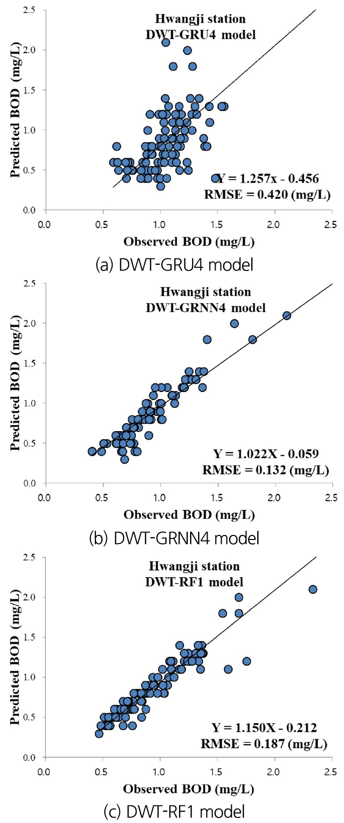
To approve the efficiency of optimum models using visual aid, Figs. 11(a)~11(c) give the scatter diagrams for observed and predicted BOD concentration values using the optimum two-stage hybrid models at Hwangji station. The values of RMSE index and linear equations for the optimum two-stage hybrid models were arrayed for corresponding scatter diagram. It can be shown from RMSE values that an apparent difference can be revealed among the DWT-GRU4, DWT-GRNN4, and DWT-RF1 models. As a result, the DWT-RF1 model carried out better than DWT-GRU4 and DWT-GRNN4 models undoubtedly, while the DWT-GRU4 model yielded the worst efficiency at Hwangji station.
4.3 Discussion
Overall, the addressed investigation investigated the nonlinear and nonstatic performance of BOD concentration using the independent and two-stage hybrid models at Dosan and Hwangji stations, South Korea. Since Dosan (GRU1, GRNN4, and RF5 models) and Hwangji (GRU4, GRNN5, and RF3 models) stations provided the best accuracy differently based on various input combinations, authors cannot confirm which input combination predicts BOD concentration among the independent models accurately. In addition, the statistical results suggested that the GRU and GRNN models could not predict BOD concentration precisely compared to the RF model based on the corresponding Division at both stations. Therefore, the predicted accuracy of independent models fluctuated for various input combinations, generally because all independent models implemented the different inferences and architectures.
The core purpose for implementation of two-stage hybrid model which combines discrete wavelet transform approach into the independent model, is to improve the predicted accuracy of BOD concentration compared to the corresponding independent model. From the viewpoint of two-stage hybrid models’ performance based on RMSE values at Dosan station, the DWT-GRU2 (2.5% for GRU2) and DWT-GRU5 (6.6% for GRU5) models enhanced the predicted accuracy clearly among the DWT-GRU models. Also, the DWT-RF1 (68.3% for RF1), DWT-RF2 (11.4% for RF2), DWT-RF3 (16.7% for RF3), and DWT-RF5 (10.2% for RF5) models boosted the predicted correctness definitely among the DWT-RF models. However, the DWT-GRNN models could not increase the predicted efficiency for corresponding GRNN models. Recognizing the optimal models’ classification for independent and two-stage hybrid models, the DWT-RF5 model, which provided the best accuracy, improved the predicted accuracy by 200.9% (DWT-GRNN4), 207.4% (DWT-GRU5), 10.2% (RF5), 125.9% (GRNN4), and 192.6% (GRU1), respectively.
Considering the two-stage hybrid models’ performance based on RMSE values at Hwangji station, the DWT-GRNN2 (36.6% for GRNN2), DWT-GRNN3 (17.4% for GRNN3), DWT-GRNN4 (87.9% for GRNN4), and DWT-GRNN5 (19.1% for GRNN1) models boosted the predicted efficiency obviously among the DWT-GRNN models. In addition, only the DWT-RF1 (43.9% for RF1) increased the predicted efficiency clearly among the DWT-RF models. However, the DWT-GRU models could not improve the predicted efficiency for corresponding GRU model. Regarding the optimal models’ classification for independent and two-stage hybrid models, the DWT-GRNN4 model which yielded the best efficiency, increased the predicted efficiency by 41.7% (DWT-RF1), 218.2% (DWT-GRU4), 23.5% (RF3), 41.7% (GRNN5), and 177.3% (GRU4), respectively. In this investigation, the two-stage hybrid models could not always enhance the predicted accuracy of independent model at both stations. This demonstration followed the previous article of Zounemat-Kermani et al. (2019) similarly, which developed the multilayer perceptron (MLP) and cascade correlation neural networks (CCNN) models to predict DO concentration in Florida, USA. They combined two data pre-processing approaches including DWT and variational mode decomposition (VMD) into the MLP and CCNN models for enhancing the predicted accuracy of DO concentration. Results revealed that the DWT-CCNN and VMD-CCNN models could not improve the predicted accuracy of CCNN model. Kim et al. (2020) provided the deep echo state network (Deep ESN), extreme learning machine (ELM), gradient boosting regression tree (GBRT), and RF models to predict BOD concentration at Gongreung and Gyeongan stations, South Korea. They found that the Deep ESN model accomplished the most accurate prediction among the developed standalone models.
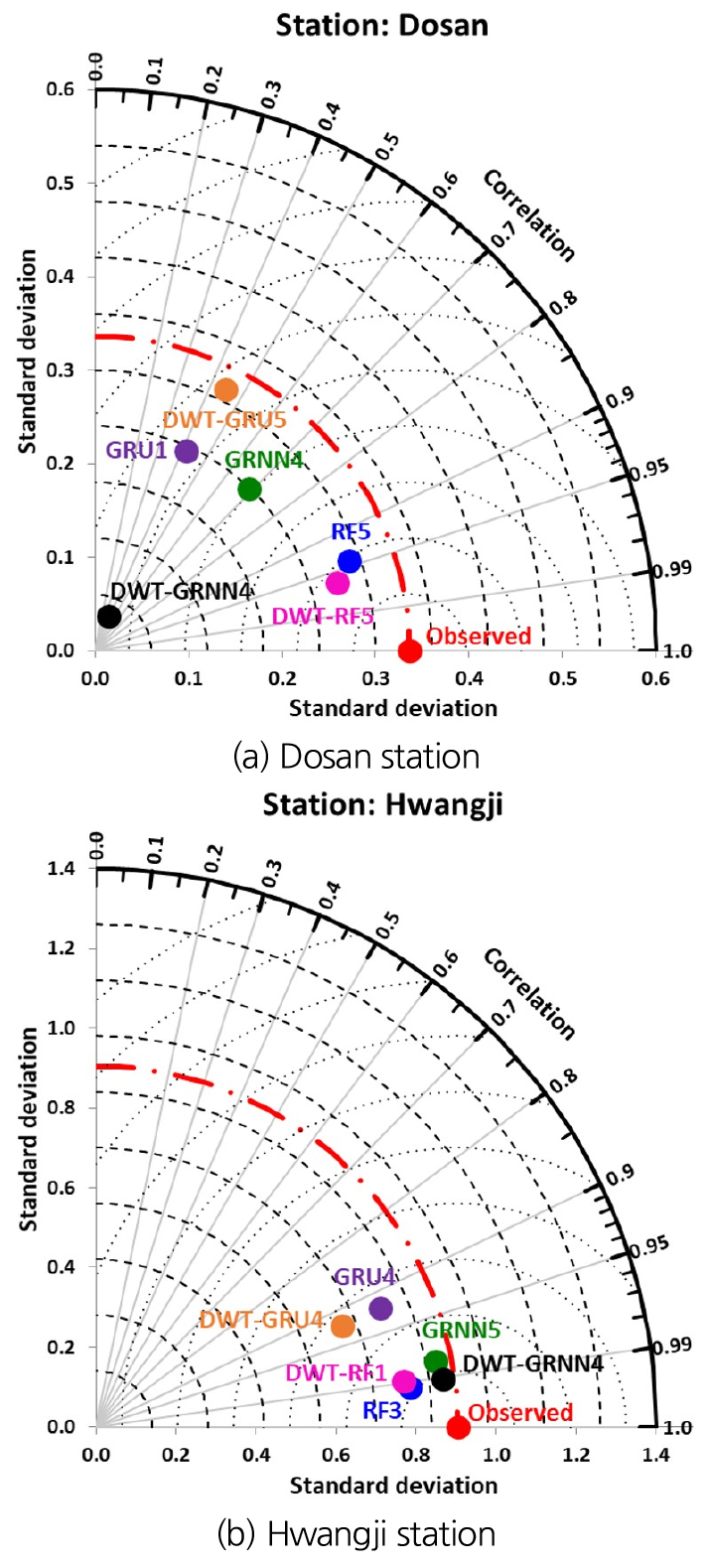
Taylor (2001) implemented the polar-based scheme to acquire a visual assistance of model accomplishment. He described that the addressed special scheme explained the relationship of three statistical indices including CC, normalized standard deviation (NSD), and RMSE obviously. Fig. 12(a) provides the Taylor scheme based on the optimal independent and two-stage hybrid models for Dosan station. It can be found from Fig. 12(a) that the points of RF5 and DWT-RF5 (i.e., has the smallest RMSE) models signified the shortest from the observed one, whereas the points of GRU1 and DWT-GRNN4 models displayed the longest visualization from that of observation. Also, Fig. 12(b) illustrates the Taylor scheme based on the optimum independent and two-stage hybrid models for Hwangji station. It can be judged from Fig. 12(b) that the nodes of RF3 and DWT-GRNN4 (i.e., has the smallest RMSE) models indicated the nearest from the measured one, while the nodes of GRU4 and DWT-GRU4 models proved the longest distances from that of measurement.
Since this investigation may not be conventional and traditional approach to predict BOD concentration, their limitation should be investigated by future tasks. Therefore, the paradigm which combines the different evolutionary algorithms (Sahay and Srivastava, 2014; Kalteh, 2015; Yaseen et al., 2018; Zakhrouf et al., 2018, 2020; Fallah et al., 2019; Rezaie-Balf et al., 2019) into the two-stage hybrid models, is recommended to enhance the predicted accuracy of BOD concentration.
5. Conclusions
This investigation surveyed the predicted accuracy and efficiency of BOD concentration utilizing the independent and two-stage hybrid models at Dosan and Hwangji stations, South Korea. Among eleven water quality and quantity indicators available from both stations, eight water quality and quantity indicators including pH, WT, SS, COD, T-P, TOC, BOD, and DIS were selected to constitute the various input combination (i.e., Divisions 1-5). For the training and testing steps of independent and two-stage hybrid models, the collected data (January 2008 - December 2020) were separated into 80% (training) and 20% (testing), respectively. The statistical criteria and graphical support (i.e., scatter diagram and Taylor scheme) were employed to compare the discussed models based on various input combinations.
Considering the best models from all Divisions 1-5, the DWT-RF5 model (RMSE = 0.108 mg/L, NSE = 0.897, and CC = 0.960) provided the best results compared to the discussed optimal models (i.e., GRU1, GRNN4, RF5, DWT-GRU5, and DWT-GRNN4) based on independent and two-stage hybrid models during testing step at Dosan station. In addition, the DWT-GRNN4 model (RMSE = 0.132 mg/L, NSE = 0.979, and CC = 0.990) was found to support the more accurate and credible results among the addressed optimum models (i.e., GRU4, GRNN5, RF3, DWT-GRU4, and DWT-RF1) for predicting BOD concentration during testing step at Hwangji station. However, this investigation demonstrated that the accuracy and efficiency of BOD concentration predicted by the independent model could not be always strengthened from the implementation of two-stage hybrid models at both stations. To confirm the results of this investigation, therefore, it must be obtained the reliable water quality and quantity indicators from the potential datasets, and accomplished the prediction of BOD concentration employing diverse two-stage hybrid paradigm in rivers.
