

1. 서 론
2. Materials and Methods
2.1 Study stations and data collections
2.2 Frost event prediction models
2.3 Model evaluation
3. Results and Discussion
3.1 Changes in frost days and frost-free period
3.2 Model evaluation
4. Summary and Conclusions
1. 서 론
It is generally accepted that late-spring frost events may damage fruit crops, while upland crops such as vegetable crops are prone to be damaged from early-fall frost events in the Republic of Korea (Hereafter South Korea). Frost events based on the heat-transfer processes can be classified into two types: radiative frosts and advective frosts (Chevalier et al., 2012; Kalma et al., 1992; Snyder et al., 1987; Temeyer et al., 2003). Radiative frosts occur due to radiational cooling under the meteorological conditions of clear skies, no wind, and a low dew point temperature. However, advective frosts occur when warmer air in a region is replaced with cold air by advection. This type of frosts tends to occur under the meteorological conditions of cloudy skies, moderate to strong winds, no temperature inversion, and low humidity. The former is more common than the latter (Temeyer et al., 2003).
Various meteorological variables have been characterized and used to develop frost event prediction models. Kwon et al. (2008) selected the eight meteorological variables related with frost occurrence. These variables are minimum temperature (denoted as Tmin), grass minimum temperature (denoted as Tmin_gr), dewpoint temperature (denoted as Dew), and wind speed (denoted as Wind) at frost days, mean relative humidity (denoted as RHmean), minimum relative humidity (denoted as RHmin), and total cloud amount (denoted as Cloud) at one day before frost days, and difference between maximum temperature at one day before frost days and minimum temperature at frost days (denoted as Tdiff). Lee et al. (2016) used these eight meteorological variables to develop frost event prediction models by logistic regression and decision tree methods in spring. They reported that Tmin, Tmin_gr, and Dew were the most selected variables from the logistic regression method, while Tmin_gr and Wind were most selected from the decision tree method. Chevalier et al. (2012) developed a web-based fuzzy expert system for frost warnings providing the five general warnings based on air temperature, Dew, and Wind. Rozante et al. (2020) developed a frost index using the five meteorological variables: temperature and relative humidity at 2m, wind speed at 10m, mean sea-level pressure, and cloudiness. Han et al. (2009) reported that cloud, temperature and cumulative rainfall amount for past 5 days were selected for the frost event prediction at Naju (South Korea) using the discriminant analysis, while Kim et al. (2017) found that the rainfall amount was less related to frost events. Kim et al. (2017) also suggested that the inclusion of Tmin_gr for the development of frost event prediction models may contribute to more accurate predictions.
Even though various machine learning techniques including logistic regression and random forest methods have been applied to predict frost event predictions, to the best of our knowledge, few studies have been conducted on a comparative assessment of frost event prediction models using machine learning and deep learning techniques. The objectives of this study were (1) to investigate changes in frost days and frost-free seasons, (2) to develop frost event prediction models using logistic regression (LR), random forest (RF), and long short-term memory (LSTM) networks, and (3) to comparatively assess these models.
2. Materials and Methods
2.1 Study stations and data collections
Lee et al. (2016) developed frost event prediction models for the six frost monitoring stations using logistic regression and decision tree techniques. However, their study was limited to a single season (i.e, spring) and recent trends in frost events were not included since the study period was from 1973 to 2014. We extended the study period up to the year 2019 to represent recent trends in frost events and aimed to develop the frost event prediction models for spring and fall since both late frosts in spring and early frosts in fall may damage crops. Unfortunately, the Chuncheon (stopped on Sept. 30, 2016), Seosan (stopped on Oct. 31, 2017), and Jinju stations (stopped on Jan. 21, 2015) were excluded in this study, because meteorological events including frost were not monitored any more at the three stations. The three frost monitoring stations such as Suwon (119), Cheongju (131), and Gwangju (156) used in this study are displayed in Fig. 1.
In this study, spring seasons were defined as March to May, while fall seasons were defined as September to November. The statistical summary of the eight meteorological variables, which were used to investigate meteorological conditions at frost days by Kwon et al. (2008), are summarized in Table 1. Tmin, Tmin_gr, and Dew at the frost days at the stations in spring (-1.1, -5.8, and -2.5℃, respectively) were generally lower than those in fall (-0.1, -4.3, and -0.6℃, respectively), while Wind and Cloud at the frost days were slightly higher in spring (1.9 m s-1 and 30.0%, respectively) than in fall (1.3 m s-1 and 27.9%, respectively). Tmin at the frost days ranged from -12.0 to 8.6℃ and from -11.0 to 7.2℃ for spring and fall, respectively, while these ranges for Tmin_gr were found to be slightly lower (-17.4 to 5.3℃ and from -17.2 to 3.1℃ for spring and fall, respectively). The ranges for temperatures including Tmin, Tmin_gr, and Dew in spring are not different from those of Lee et al. (2016). However, the maximum Tdiff values for the study period are slightly lower than those of Lee et al. (2016).
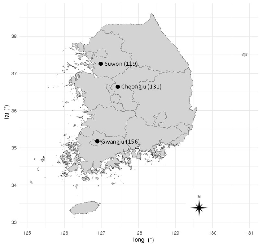
Table 1.
Statistical summary of meteorological variables at frost days at the frost monitoring stations in spring and fall for the period of 1973-2019
2.2 Frost event prediction models
In this study, scikit-learn was used for logistic regression (LR) and random forest (RF) techniques, while TensorFlow was used for the LSTM network. Scikit-learn is a Python module integrating a variety of machine learning algorithms (Pedregosa et al., 2011). The most relevant features among the eight meteorological variables were selected based on importance weights in LR and RF techniques. TensorFlow supports a wide range of application with deep neural networks (Abadi et al., 2015). The datasets from 1973 to 2010 were used for the training period, while the rest of the datasets were used for the test period. Additionally, for the LSTM network, the training period was split into two: training and validation periods (50:50). More detailed information on each method was presented in the following sections.
2.2.1 Logistic regression
LR is a common statistical method used in environmental, atmospheric, and earth sciences (Kleinbaum et al., 2002). LR was developed based on the relationship between a dependent variable and multiple independent variables (Lee, 2005). LR can estimate the probability of presence and absence using the observed values of the predictor variables (Ozdemir, 2011). From this binary nature, LR can be used to predict frost event occurrences. For example, Lee et al. (2016) developed frost event prediction models using LR. This method yields the coefficient for each variable that serves as the weights in the algorithm (Hosmer Jr et al., 2013). These weights can be used to interpret a trained model. In addition, LR can be applied for both continuous and categorical datasets compared with linear regression and log-linear regression, and generally, this method does not require the assumption of normality (Ozdemir, 2011). The general form of logistic regression can be expressed as follows:
where, are the explanatory variables, y is the dependent variable, and are the regression coefficients to be estimated. Pr indicates the probability of the occurrence of data (Hosmer Jr et al., 2013).
2.2.2 Random forest
The RF method was developed based on model aggregation suggested by Breieman (Breiman, 2001; Naghibi et al., 2016). RF is an ensemble method which consists of a combination of tree predictors. Each tree separates all instances of the dataset into two subgroups by checking all possible cases and selecting the best case to split (Xue et al., 2013). All instances and subgroups can be defined as child nodes or parent nodes. Child groups that are produced in a previous step can further be designated as a parent node. This process continues until all instances are trained (Xue et al., 2013). The RF model uses a bagging technique for a bootstrapped sample that is randomly generated based on the data. A set of bootstrapped samples is randomly generated from a training dataset, an out-of-bag (OOB) dataset then remains. Each tree is grown for each bootstrapped sample to build a set of trees. The tree is tested with the OOB data for a new prediction when a tree is grown. Finally, the RF is built by averaging the prediction of all trees (Breiman, 2001). However, a very deep classification tree often leads to overfitting on a training dataset. We set the maximum depth to be 3 considering the results by Lee et al. (2016) to reduce this overfitting problem in this study.
2.2.3 LSTM
LSTM is a popular model in recurrent neural network, which was specialized to extract the features from the sequence data (Hochreiter and Schmidhuber, 1997). LSTM consists of three “gates” (forget, input, and output gates) and two “states” (cell and hidden states). The gates are used for what information to forget (forget gate), allow in (input gate), and allow out (output gate) from the LSTM memory. The states are performed as a memory (cell state) or information carrier across time (hidden state). The equations of gates and states are as follows:
where, Cc<t> is the vector of cell state a<t-1>, is the activation function at time step t, x<t> is the input at current step t, δ is an element-wise non-linear activation function, Γf is the input gate, Γo is the forget gate, Γu is the output gate, and c<t> is a cell state at current step t. The bias and weight matrices are indicated as b and W, respectively. In this study, 1000 of epoch number and 128 of batch size were assigned and the learning rate was 0.001. For the binary nature, the sigmoid function and the binary cross-entropy loss function were employed as the activation function and the loss function, respectively, in this study. The input data of LSTM adopted the eight meteorological variables at previous time steps: <t-10>, <t-5>, and <t-1>. However, the differences in area under the Receiver Operating Characteristic (ROC) curve (AUC) from those time steps were very small (data not given). Therefore, only <t-1> time step was considered in this study.
2.3 Model evaluation
The frost event prediction models were evaluated using Precision (P), Recall (R), and f-1 scores. These scores can be calculated by Eqs. (10) ~ (12) for P, R, and f-1, respectively and all terms in those equations can be found in the confusion matrix (Table 2). For this study, P was defined as the ratio of correctly predicted frost events (TP) to the total predicted frost events (TP + FP), while R was defined as the ratio of correctly predicted frost events (TP) to the total frost events in observations (TP + FN). The f-1 score was defined as the harmonic mean of the P and R. These three scores can vary with the range of 0 (the poorest value) to 1 (the perfect score). The Receiver Operating Characteristic (ROC) curve and reliability diagram were additionally used to evaluate the frost event prediction models. A convex shape of the ROC curves to the top-left corner of the plot indicates a skillful forecast system and the diagonal line in the plot indicates “no-skill”, while in the reliability diagram, the diagonal line indicates “perfect reliability”.
3. Results and Discussion
3.1 Changes in frost days and frost-free period
Fig. 2 shows the frequency of frost occurrence at Suwon (119), Cheongju (131), and Gwangju (156) in spring and fall for the period of 1973-2019. The mean of frequencies of frost occurrence at Suwon, Cheongju, and Gwangju in spring (fall) for this period were 18(16), 15(17), and 12 days (9 days), respectively. The highest frost days in spring were observed at Suwon with the range from 2 to 34 days, while the most was observed at Cheongju in fall (Figs. 2(b) and 2(d)). Significant decreases in trends (p < 0.01) were also observed at all stations in both spring and fall. The trend rates were -4.49(-3.37), -5.56(-4.06), and -2.25 days (-1.22 days) per decade at Suwon, Cheongju, and Gwangju in spring (fall), respectively. Similar decreasing trends of frost days in the United States were found in the results of Easterling (2002). Unlike these results, Easterling (2002) reported significant decreasing trends of frost days in the United States in spring but no significance in fall. Higher trend rates at all stations were found in spring than those in fall.
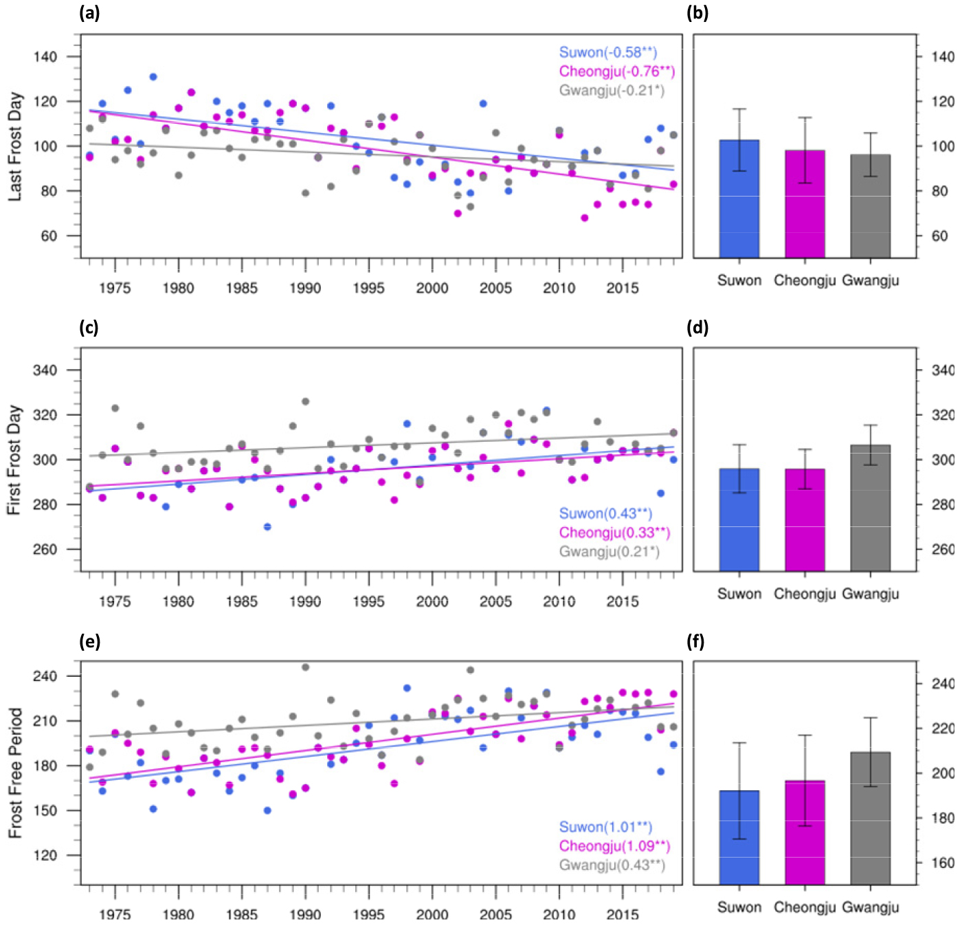
Fig. 3 displays the time series and linear trends, and mean with one standard deviation for the dates of the last-spring frost, first-fall frost, and the length of the frost-free period. The dates were converted to the Julian days (i.e., days of the year) before the calculation. There was a decrease in the last frost day, and the decreasing trend was largest at Cheongju (-0.76 day year-1), followed by Suwon (-0.58 day year-1) and Gwangju (-0.21 day year-1). The mean and standard deviation of the last frost day was 102.8 and 13.8 days at Suwon, 98.1 and 14.5 days at Cheongju, and 96.2 and 9.6 days at Gwangju, respectively. The mean of last frost day was latest at Suwon on around April 12-13 and on around April 8-9 at Cheongju and on around April 6-7 at Gwangju for the period of 1973-2019.
On the other hand, there was an increase in the first frost day, and the increasing trend was largest at Suwon (0.43 day year-1), followed by Cheongju (0.33 day year-1) and Gwangju (0.21 day year-1). The mean and standard deviation was 295.9 and 10.7 days at Suwon, 295.8 and 8.8 days at Cheongju, and 306.5 and 8.9 days at Gwangju, respectively. The mean of first frost day was latest at Gwangju on around November 2-3, while that was same at Suwon and Cheongju on around October 22-23 for the period 1973-2019. These results represent that the last frost day in spring is occurring earlier, whereas the first frost day in fall is occurring later. Subsequently, the increasing trends of the frost-free period (1.01 day year-1 at Suwon, 1.09 day year-1 at Cheongju, and 0.43 day year-1 at Gwangju) were observed. These longer frost-free season and decreasing frost days are in substantial agreement with other studies (e.g., Bonsal et al., 2001; Frich et al., 2002; Heino et al., 1999).
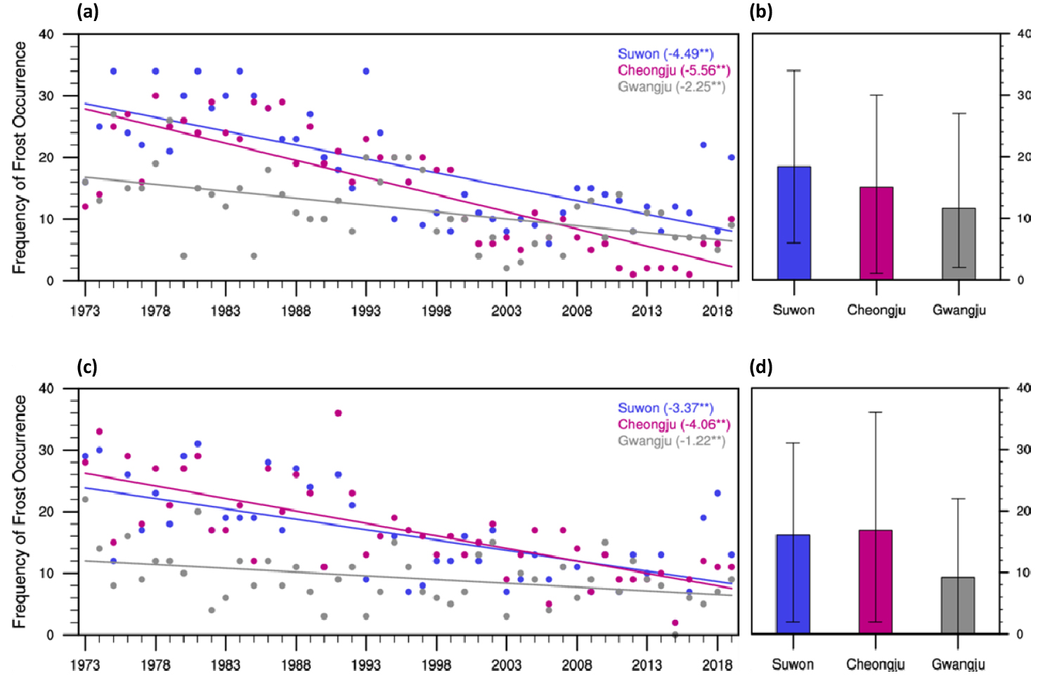
Fig. 2.
Frequency of frost occurrence at the frost monitoring stations in a) spring and (c) fall for the period of 1973-2019 and (b, d) mean with standard deviation. The lines indicate the linear trends. The * and ** indicate statistical significance at the 0.05 and 0.01 probability levels, respectively
3.2 Model evaluation
For LR and RF, important explanatory variables were selected using the sklearn.feature_selection module (Pedregosa et al., 2011). Tmin, Tmin_gr, and Wind were selected in common at all stations in both the spring and fall seasons for LR, while for RF, Tmin, Tmin_gr, and Dew were selected in common at all sites in both the spring and fall seasons. These explanatory variables were also selected variables in the results by Lee et al. (2016). However, for RF, Wind was also selected at the three stations in their results. This explanatory variable (Wind) was not selected in this study. Instead, Dew was considered as a more important explanatory variable in this study. These variables were those (Tmin, Tmin_gt, Dew, and Wind) at frost days among the eight meteorological variables that Kwon et al. (2008) analyzed for frost events. These results imply that these variables more contributed to the frost events at the stations than those at one day before frost days. These variables have been selected for the frost event prediction in many studies (e.g., Ding et al., 2019; Temeyer et al., 2003). The simulated and observed seasonal frost events are displayed in Fig. 4. Overall, the random forest method better performed the number of seasonal frost events at the three stations in both spring and fall for the training period than the other two methods. For the training period, the other two methods tended to underestimate the number of seasonal frost events in spring, while those slightly overestimated the number of seasonal frost events in fall except for the Gwangju station. At the Gwangju station in fall, the number of seasonal frost events were slightly underestimated in the 2000s (Fig. 4(f)). However, decreasing trends in frost events at all stations in both spring and fall were clearly seen for the entire period. These results are in good agreement with previous studies by Xiao et al. (2018) and Vitasse et al. (2018). Xiao et al. (2018) and Vitasse et al. (2018) showed that warming temperature can reduce frost events. However, they also reported that in spite of increases in temperature, the risk of frost damage was not reduced. This can be explained by considering that an increase in temperature may accelerate crop phenology in spring (Sgubin et al., 2018; Vitasse et al., 2018; Xiao et al., 2018).
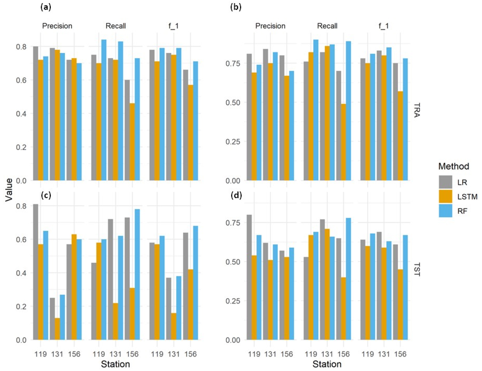
P, R, and f-1 scores are displayed in Fig. 5. The R scores from RF were higher than those from the other two methods except for the Cheongju station for the test period in fall. For both the training and test periods, R scores from the LSTM method at the Gwangju station in both spring and fall were smaller than P scores. This result indicates that frost events in the observations predicted as not frost events (false negative) by the LSTM method at the Gwangju station were large and incorrectly predicted frost events (false positive) were small. This result showed the inverse relationship between P and R scores. For this case at the Gwangju station, the f-1 scores can be a useful metric, since the f-1 score is the harmonic mean of P and R reflecting the P-R trade-off. Therefore, when we evaluated the three model performances based on the f-1 scores, these results showed that the LSTM performances were lowest.
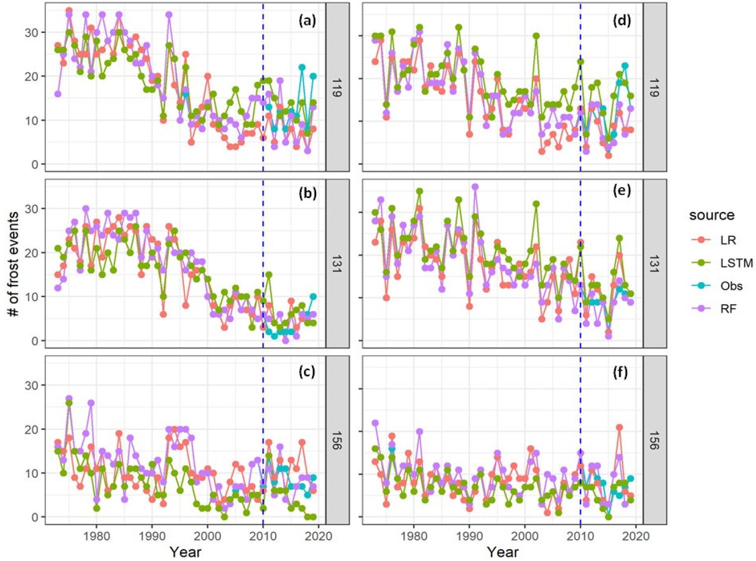
Fig. 4.
Comparisons of the observed and simulated numbers of frost occurrences at (a, d) Suwon (119), (b, e) Cheongju (131), and (c, f) Gwangju (156) in spring (a-c) and in fall (d-f). The left-hand side of the vertical blue dashed line indicates the training period and the right-hand side of it indicates the test period
For the training period, AUC varied with the range of 0.94 to 0.97 in spring, while the range of the AUC values were 0.95 to 0.98 in fall (Fig. 6). Based on these AUC values, RF slightly better performed to predict frost events than the other two methods. The AUC values for LSTM were lowest at all stations. For the test period, the AUC values of the LSTM were somewhat lower than those for the training period, whereas those of RF were slightly higher than those for the training period (Fig. 7). Similar results to this were found in the reliability curves. The slopes of the reliability curves for the training period were close to the perfect reliability line (i.e., the diagonal line in Fig. 8) in both spring and fall. However, this high reliability was not shown in the reliability curves for the test period (Fig. 9). Especially, the curves were very far from the diagonal line above 0.5 of mean predicted value at the Cheongju station (Figs. 9(b) and 9(e)). This indicates that the results from the frost event prediction models were not very reliable, because as forecast probability increased from approximately 0.8 to 1.0, the actual chance of observing the frost event decreased from about 0.5 to 0.4 (Fig. 9(e)). A further study is recommended on the improvement of reliability of the frost event prediction models.
The observed and simulated first frost days, last frost days, and frost-free period are summarized in Table 3. The simulated last frost days were earlier than the observed last frost days at the three stations. The differences between the observed and simulated first frost days were smaller than those for the last frost days. For the frost-free periods, the largest differences were simulated by LR at the three stations. Since these first and last frost days could result in frost damages to crops, it is important to accurately predict those first and last frost days to reduce the frost damages to crops. Even though the frost prediction models showed very high predictability with above 0.9 of AUC, these models did not accurately predict those first and last frost days. These results suggest a further study on the improvement of the predictability of the first and last frost days.
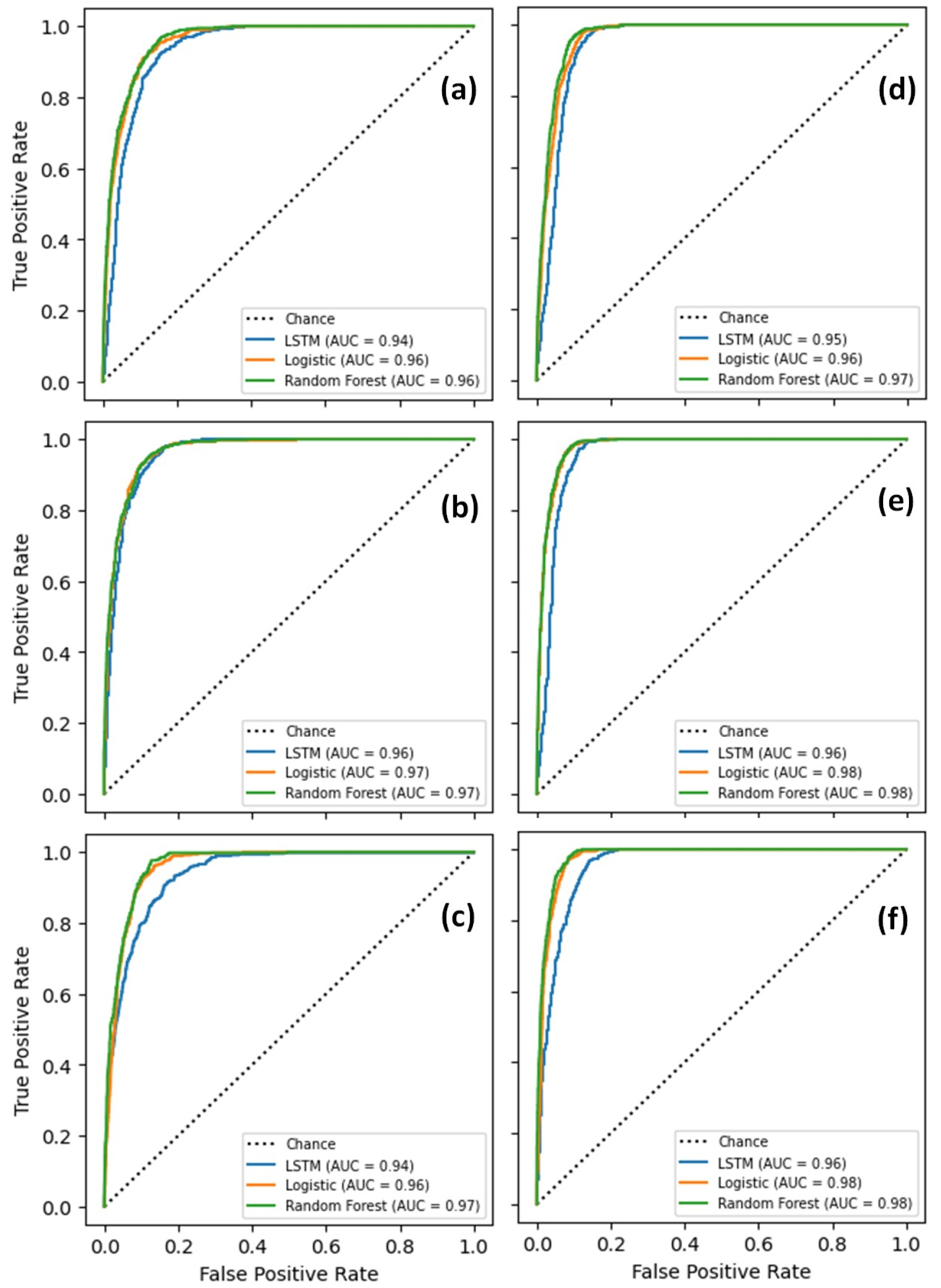
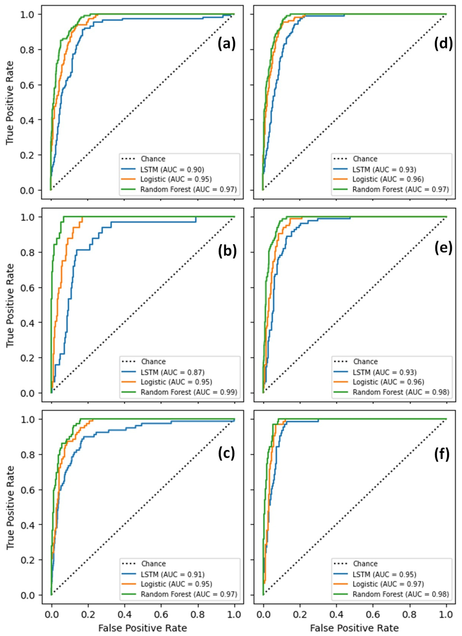
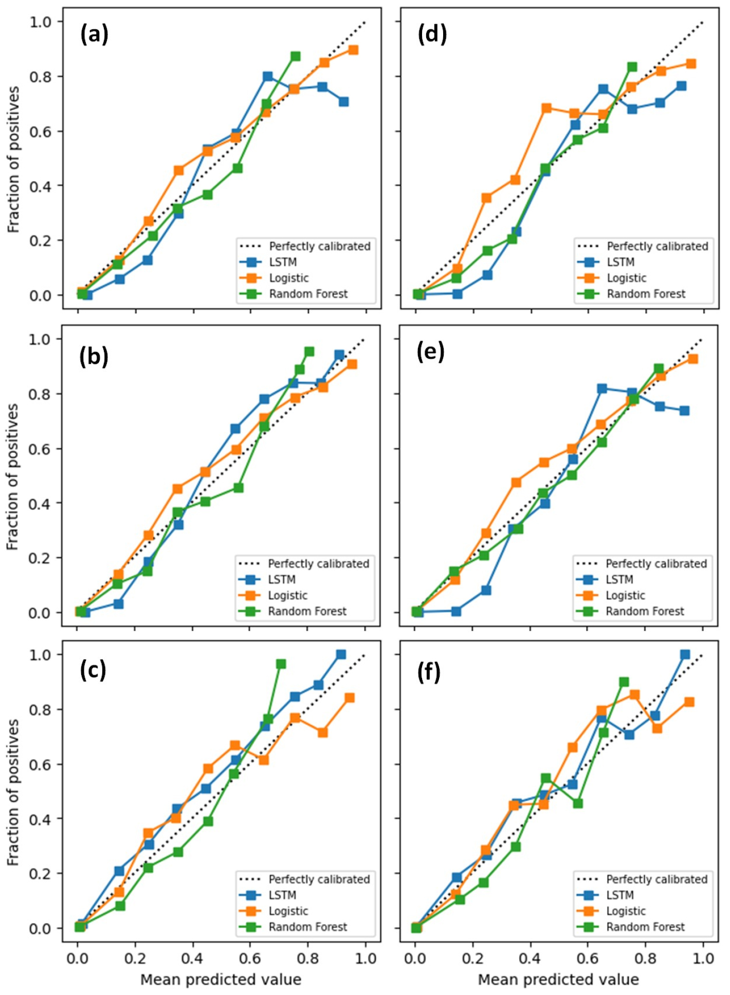
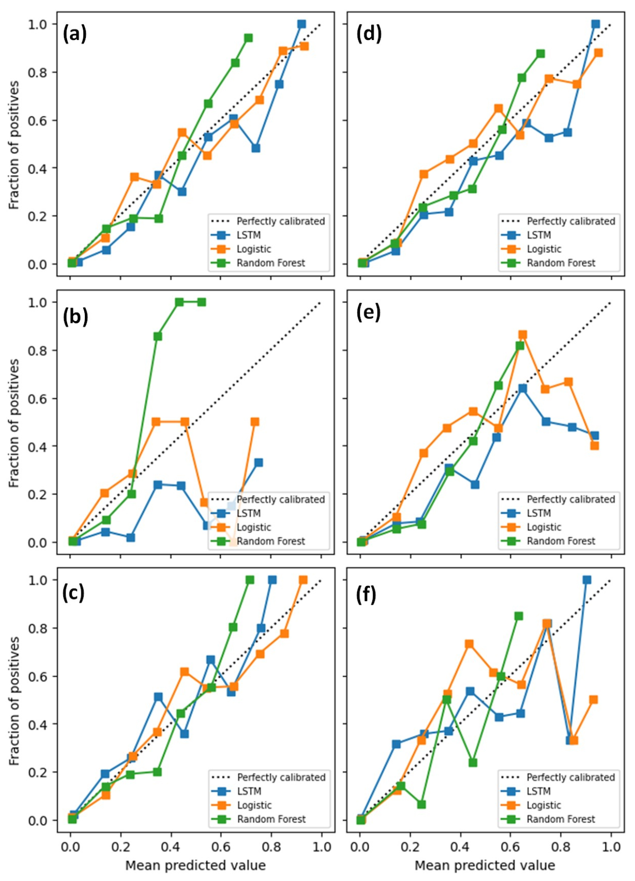
Table 3.
Statistical summary of the observed and simulated first frost days, last frost days, and frost-free period at the frost monitoring stations for the period of 1973-2019
4. Summary and Conclusions
We investigated changes in frost days and frost-free periods and comparatively assessed the frost event prediction models using logistic regression, random forest, and long short-term memory networks. Tmin, Tmin_gr, Dew, and Wind at frost days, RHmean, RHmin, and Cloud at one day before frost days, and Tdiff were collected from the three stations (Suwon, Cheongju, and Gwangju) for the period of 1973-2019 and used to develop the frost event prediction models. In this study, we found the followings:
1) The results showed that significant decreasing trends in the frequencies of frost days at the three stations in both spring and fall.
2) The last frost days in spring were getting earlier, while the first frost days in fall were getting later, suggesting longer frost-free periods.
3) Minimum temperature and grass minimum temperature were the most selected explanatory variables in both LR and RF.
4) Overall, the three-evaluation metrics (P, R, and f-l score) showed that the performance of RF was highest, while that of LSTM was lowest.
5) In spite of higher AUC values at the three stations, low reliability at the Cheongju station was observed and the accuracy of the first frost days and last frost days were not very high.
This study recommends a further study on the improvement of the predictability of both frost events and the first and last frost days and reliability of the frost event prediction models.
